Linear markets
Lines
A demand or supply curve is a straight line in inverse form:
where \(a\) is the price intercept and \(b\) the slope (\(b < 0\) for demand, \(b > 0\) for supply). Price is always on the vertical axis and quantity on the horizontal one, following Marshall (1890). Discrete unit schedules (Discrete markets) and market curves summed from individual curves (Market curves from individuals) are not single straight lines.
Line.from_inverse(float, float)
Line.from_standard(
    float,
    float,
    float
)Price at quantity \(q\).
Quantity at price \(p\).
Price at \(Q = 0\) (the choke price of a demand curve).
Quantity at \(p = 0\).
\(\mathrm{d} p / \mathrm{d} Q\).
(a, b) for \(p = a + b Q\).
A new line with delta_intercept (\(\Delta a\)) added to the intercept and delta_slope (\(\Delta b\)) added to the slope.
A straight line in the price--quantity plane, stored as
\(A p + B Q + C = 0\) so that horizontal and vertical lines are allowed.
from_inverse(a, b) builds \(p = a + b Q\); from_standard(A, B, C) builds
\(A p + B Q + C = 0\). The package root also exports the two constructors as
line_from_inverse() and line_from_standard().
from principle_viz import line_from_inverse, line_from_standard

demand = line_from_inverse(10.0, -1.0)
# 6.0 7.0
print(demand.q_at(4), demand.p_at(3))
# 10.0 10.0
print(demand.p_intercept(), demand.q_intercept())
# (10.0, -1.0)
print(line_from_standard(1, 1, -10).to_inverse())
\((A, B, C) = (1, 1, -10)\) is equivalent to \(p = 10 - Q\).
A horizontal line has no \(Q(p)\) and a vertical line has no \(p(Q)\); the
corresponding methods raise NonInvertibleLineError.
Equilibrium
solve_equilibrium(demand, supply)The intersection of two lines, returned as an EquilibriumResult
(Quick start). Parallel lines raise ParallelLinesError, identical
lines CoincidentLinesError.
from principle_viz import solve_equilibrium

eq = solve_equilibrium(demand, line_from_inverse(2.0, 1.0))
print(eq)
# EquilibriumResult(q_star=4.0, p_star=6.0,
#                   is_valid_market=True, notes=())
\(10 - Q = 2 + Q\) gives an equilibrium quantity of 4 and an equilibrium price
of 6; is_valid_market is True and notes is empty.
Comparative statics
ShiftSpec(delta_intercept=0.0, delta_slope=0.0)
ShiftScenario(demand_shift=None, supply_shift=None)
A shift of one curve in inverse form: delta_intercept moves it up
(\(> 0\)) or down, delta_slope rotates it. A scenario shifts demand,
supply or both. Both live in principle_viz.core.shifts.
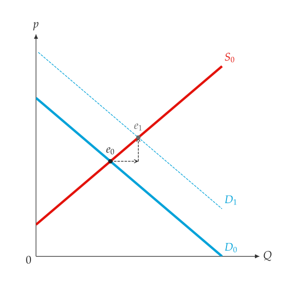
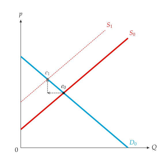
An increase in demand raises the demand intercept; an increase in supply lowers the supply intercept, since sellers accept a lower price at every quantity.
comparative_statics(
    demand,
    supply,
    scenario
)The EquilibriumResult before the shift.
The EquilibriumResult after the shift.
The baseline and shifted lines (baseline_demand, shifted_demand, ...).
Change in quantity.
Change in price.
Direction of the quantity change: "left" or "right" ("none" when unchanged).
Direction of the price change: "up" or "down" ("none" when unchanged).
Solve the market before and after the shift. The result has these fields:
from principle_viz import comparative_statics
from principle_viz.core.shifts import ShiftScenario, ShiftSpec

up = ShiftScenario(demand_shift=ShiftSpec(delta_intercept=3.0))
result = comparative_statics(demand, supply, up)
new = result.shifted_equilibrium
# 5.5 7.5
print(new.q_star, new.p_star)
# right up
print(result.direction_q, result.direction_p)
MarketFigure.add_comparative_statics(
    result,
    q_max,
    *,
    demand_label="$D_1$",
    supply_label="$S_1$"
)
Draw the curve that moved, both equilibria and dashed arrows from the old
equilibrium to the new one. Name the original curves \(D_0\) and \(S_0\) in
add_curves(). An increase in demand is shown in An increase in demand. and a
decrease in supply in A decrease in supply..
fig = MarketFigure(
    x_max=12, y_max=14, title="Increase in Demand"
)
fig.add_curves(
    demand,
    supply,
    q_max=10,
    demand_label="$D_0$",
    supply_label="$S_0$",
)
fig.add_comparative_statics(result, q_max=10)
fig.finalize()
Errors
Every exception the package raises derives from PrincipleVizError, in
principle_viz.exceptions; catching it handles all of them.
PrincipleEconError, the name before 0.10.0, is the same class. Exceptions
lists when each exception is raised.
A line cannot be built or transformed
A horizontal line is asked for \(Q(p)\), or a vertical one for \(p(Q)\)
Demand and supply never meet
Demand and supply are the same line
A tax, subsidy, control or trade scenario is invalid
A discrete schedule is invalid (Discrete markets)
Individual curves cannot be summed, or a price is outside a piecewise curve (Market curves from individuals)
A production possibilities frontier is invalid (Production possibilities)