Production possibilities

ProductionPossibilitiesFrontier(
    x_intercept,
    y_intercept,
    curvature=1.0,
    x_good="Good X",
    y_good="Good Y"
)

y_at(x)

Output of \(y\) when \(x\) units of the first good are produced.

opportunity_cost_x(x)

Units of \(y\) given up for one more unit of \(x\), \(\left| \mathrm{d} y / \mathrm{d} x \right|\).

assess(x, y)

A PointStatus: EFFICIENT on the frontier, INEFFICIENT inside it, UNATTAINABLE outside.

The frontier

\[ y = Y (1 - (x / X)^c), \]

through the intercepts \(X\) and \(Y\). A curvature \(c = 1\) gives a straight line (constant opportunity cost); \(c > 1\) bows it out (increasing opportunity cost). Intercepts and curvature must be positive and \(c \ge 1\), otherwise PPFError is raised.

from principle_viz import ProductionPossibilitiesFrontier

ppf = ProductionPossibilitiesFrontier(
    10,
    8,
    curvature=2,
    x_good="Consumer goods",
    y_good="Capital goods",
)
# 5.12 0.96
print(ppf.y_at(6), ppf.opportunity_cost_x(6))
print(ppf.assess(4, 3), ppf.assess(7, 6))
# PointStatus.INEFFICIENT PointStatus.UNATTAINABLE

analyze_ppf(
    frontier,
    points=(),
    *,
    samples=101
)
ppf_canvas(
    result,
    *,
    theme=None,
    labels=None,
    visibility=None
)

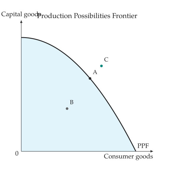
Sample the frontier and assess named points, given as (x, y, label) triples; ppf_canvas(), in principle_viz.visuals.ppf, draws it with the attainable set shaded and the points labelled (Efficient, inefficient and unattainable points.).

from principle_viz import analyze_ppf
from principle_viz.visuals.ppf import ppf_canvas

points = ((6, ppf.y_at(6), "A"), (4, 3, "B"), (7, 6, "C"))
result = analyze_ppf(ppf, points=points)
ppf_canvas(result).save("ppf_points.png")

PPFGrowthScenario(x_growth_rate=0.0, y_growth_rate=0.0)
analyze_ppf_growth(
    frontier,
    scenario,
    *,
    samples=101
)
ppf_growth_canvas(
    result,
    *,
    theme=None,
    labels=None,
    visibility=None
)

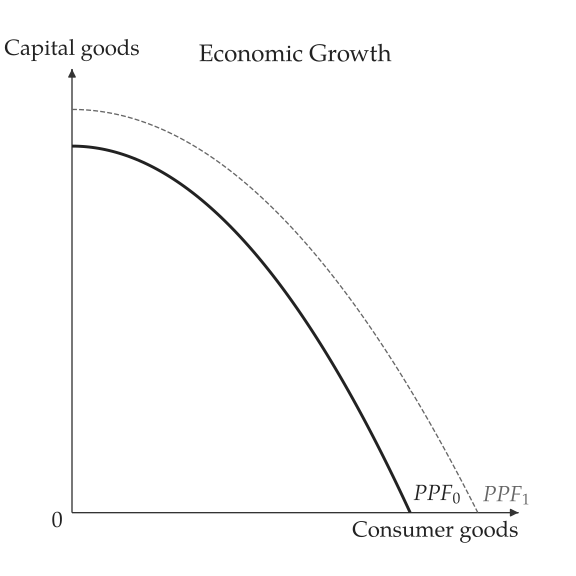
Economic growth scales each intercept by one plus its growth rate; the result holds the baseline and shifted frontiers and their sampled points. ppf_growth_canvas() draws both, named \(P P F_0\) and \(P P F_1\) (see Growth of 20% in consumer goods and 10% in capital goods.).

Comparative advantage

compare_linear_ppfs(
    name_a,
    frontier_a,
    name_b,
    frontier_b
)

For two straight-line frontiers, the opportunity cost of \(x\) for each producer and who has the comparative advantage in each good ("tie" when the costs are equal). Curved frontiers raise PPFError.

from principle_viz import compare_linear_ppfs

# x costs 0.5 y
ann = ProductionPossibilitiesFrontier(10, 5)
# x costs 1 y
bob = ProductionPossibilitiesFrontier(6, 6)
result = compare_linear_ppfs("Ann", ann, "Bob", bob)
print(
    result.comparative_advantage_x,
    result.comparative_advantage_y,
)
# Ann Bob

Ann has the comparative advantage in \(x\) (0.5 against 1) and Bob in \(y\) (1 against 2).

Comments