Labor and loanable funds
Minimum wage
analyze_minimum_wage(
    demand,
    supply,
    minimum_wage
)
A competitive labor market with a wage floor. The MinimumWageResult
has equilibrium, minimum_wage, is_binding, labor_demanded,
labor_supplied, employment (the smaller of the two),
unemployment (their gap) and wage_bill.
from principle_viz import analyze_minimum_wage

labor_demand = line_from_inverse(12, -1)
labor_supply = line_from_inverse(2, 1)
labor = analyze_minimum_wage(
    labor_demand,
    labor_supply,
    minimum_wage=9,
)
# 3.0 4.0
print(labor.employment, labor.unemployment)
MarketFigure.add_minimum_wage(
    result,
    *,
    gap_brace="line"
)
The wage floor drawn like a price floor (Price controls): the "Minimum wage" line, \(w_{\min}\) on the wage axis, and for a binding floor \(L_d\) and \(L_s\) with an "Unemployment" brace. Title the axes \(L\) and \(w\) and name the curves \(D_L\) and \(S_L\) (see A binding minimum wage.):
fig = MarketFigure(x_max=11, y_max=14, x_label="L", y_label="w")
fig.add_curves(
    labor_demand,
    labor_supply,
    q_max=10,
    demand_label="$D_L$",
    supply_label="$S_L$",
)
fig.add_minimum_wage(labor)
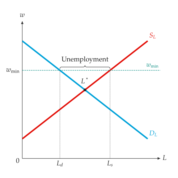
labor_demanded is 3, labor_supplied is 7, employment is 3 and
unemployment is 4.
Loanable funds
LoanableFundsScenario(
    savings_quantity_shift=0.0,
    investment_quantity_shift=0.0,
    government_borrowing=0.0
)
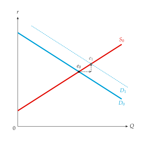
Horizontal shifts of saving (supply) and investment (demand), measured in quantity. Government borrowing (non-negative) adds to the demand for loanable funds.
analyze_loanable_funds(
    savings,
    investment,
    scenario
)
The market for loanable funds before and after the shift:
baseline_equilibrium, shifted_equilibrium, shifted_savings,
shifted_investment_demand, private_investment_after,
interest_rate_change and crowding_out, the private investment
displaced by the higher interest rate.
from principle_viz import (
    LoanableFundsScenario,
    analyze_loanable_funds,
)

savings = line_from_inverse(2, 0.5)
investment = line_from_inverse(12, -0.5)
scenario = LoanableFundsScenario(government_borrowing=4)
funds = analyze_loanable_funds(savings, investment, scenario)
# 1.0 2.0
print(funds.interest_rate_change, funds.crowding_out)
interest_rate_change is 1.0 and crowding_out is 2.0.
MarketFigure.add_loanable_funds(result)Draw the shifted curves, named \(D_1\) or \(S_1\), both equilibria and the movement between them. Title the price axis \(r\) (see Government borrowing crowds out private investment.).