Bézier curves

The Bernstein basis

Definition · Bernstein polynomials

The Bernstein polynomials of degree $n \ge 0$ are

\[ b_{i,n}(t) = \binom{n}{i} t^i (1-t)^{n-i}, \quad i = 0, \ldots, n. \]

For all other integers $i$ we put $b_{i,n} = 0$.

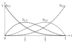
The polynomials are due to Bernstein (1912); Farouki (2012) surveys their history and properties, and The cubic Bernstein polynomials. shows the cubic ones. The proofs below use two identities of binomial coefficients.

Lemma · Binomial identities

Let $n \ge 1$ and let $i, j$ be integers, with $\binom{m}{k} = 0$ for $k < 0$ or $k > m$. Then

\[ \binom{n-1}{j} + \binom{n-1}{j-1} = \binom{n}{j} \]

and

\[ i \binom{n}{i} = n \binom{n-1}{i-1}. \]

The cubic Bernstein polynomials.

Proposition · Bernstein basis

For $n \ge 0$, the polynomials $b_{0,n}, \ldots, b_{n,n}$ are a basis of the vector space of real polynomials of degree at most $n$.

This is Theorem 1.1 of Floater (2025); Proofs proves it from scratch.

Proposition · Partition of unity

For every $t \in [0, 1]$, $b_{i,n}(t) \ge 0$ for all $i$, and

\[ \sum_{i=0}^n b_{i,n}(t) = 1. \]

Definition · Bézier curve

Let $P_0, \ldots, P_n \in \mathbb{R}^d$. The Bézier curve of degree $n$ with control points $P_0, \ldots, P_n$ is

\[ B(t) = \sum_{i=0}^n b_{i,n}(t) P_i, \quad t \in [0, 1], \]

and its control polygon is the polyline $P_0 P_1 \ldots P_n$.

The definition follows B{\'e}zier (1966) in the form of Farin (2002) and Prautzsch (2002).

Proposition · Endpoints

$b_{i,n}(0) = 1$ if $i = 0$ and $0$ otherwise; $b_{i,n}(1) = 1$ if $i = n$ and $0$ otherwise. Hence $B(0) = P_0$ and $B(1) = P_n$.

Corollary · Convex hull

Every point $B(t)$, $t \in [0, 1]$, lies in the convex hull of the control points $P_0, \ldots, P_n$.

Proposition · Affine invariance

For every affine map $A(x) = M x + v$ and every $t \in [0, 1]$,

\[ A(B(t)) = \sum_{i=0}^n b_{i,n}(t) A(P_i). \]

Transforming the curve is the same as transforming its control points.

Convex hull keeps a curve inside the region its control polygon spans, and Affine invariance is why the exporters and the Matplotlib adapter can move, scale or rotate a curve by moving its control points alone.

BernsteinBasis(int)(float)
BernsteinBasis(int).matrix(values)

The basis of one degree, in bezierkit.bezier.basis. Calling it at $t$ returns the values $b_{i,n}(t)$ for $i = 0, \ldots, n$ as an array; matrix() returns one such row per parameter value.

Curves

BezierCurve(
    points,
    *,
    evaluator=None
)
BezierCurve.linear(p0, p1)
BezierCurve.quadratic(
    p0,
    p1,
    p2
)
BezierCurve.cubic(
    p0,
    p1,
    p2,
    p3
)

degree

The degree $n$.

dimension

The dimension $d$.

control_points

The control points as a PointSet.

at()

$B(t)$ as a Point; a curve object is also callable, curve(t).

at_many()

$B$ at many parameters, as a PointSet.

evaluator

The evaluation strategy (see below).

An immutable Bézier curve of any degree $n \ge 0$ and dimension $d \ge 1$, over $[0, 1]$. points is a sequence of Points, a PointSet, a $(n + 1) \times d$ array or a ControlPolygon; the control points must share one dimension.

The operations on a curve, derivative(), split(), segment() and reversed(), are the subject of Derivatives, reversal and subdivision.

Evaluation

de Casteljau's algorithm evaluates $B(t)$ by repeated linear interpolation.

Definition · de Casteljau points

For a parameter $t$ put $P_i^{(0)} = P_i$ and, for $r = 1, \ldots, n$,

\[ P_i^{(r)} = (1 - t) P_i^{(r-1)} + t P_{i+1}^{(r-1)}, \quad i = 0, \ldots, n - r. \]

Each round averages neighbouring points, so the polygon shrinks by one point; after $n$ rounds one point is left (de Casteljau's algorithm at $t = 0.4$.). The algorithm goes back to Paul de Casteljau's work at Citroën around 1959 M{\"u}ller (2024).

Theorem · de Casteljau

For $0 \le r \le n$ and $0 \le i \le n - r$,

\[ P_i^{(r)} = \sum_{j=0}^r b_{j,r}(t) P_{i+j}. \]

In particular $P_0^{(n)} = B(t)$.

The statement is Theorems 1.6 and 1.7 of Floater (2025).

$de Casteljau's algorithm at $t = 0.4$.$

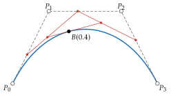
Every intermediate point is a convex combination of the control points, so the algorithm never forms large cancelling terms; it is the numerically stable choice for high degrees. Its cost is $O(n^2)$ per parameter.

DeCasteljauEvaluator

The default evaluation strategy, in bezierkit.bezier.evaluation: the algorithm above, applied to a whole batch of parameters at once with NumPy.

BernsteinEvaluator

Multiplies the Bernstein matrix by the control points. It is faster for low degrees and large batches but sums terms that can cancel at high degree. By de Casteljau both strategies compute the same polynomial.

from bezierkit import BezierCurve
from bezierkit.bezier.evaluation import BernsteinEvaluator

fast = BezierCurve(
    curve.control_points, evaluator=BernsteinEvaluator()
)
# Point(coords=(2.0, 1.5)), as with the default
print(fast.at(0.5))

The repository's benchmarks/ directory compares the two on batches of 400, 10,000 and 100,000 parameter values.

Degree elevation

A curve of degree $n$ is also a curve of degree $n + 1$; the new control points are convex combinations of neighbouring old ones.

Lemma · Degree elevation identity

For $n \ge 0$, $0 \le i \le n$ and every $t$,

\[ b_{i,n}(t) = (n + 1 - i) / (n + 1) b_{i,n+1}(t) + (i + 1) / (n + 1) b_{i+1,n+1}(t). \]

Proposition · Degree elevation

Let $B$ have control points $P_0, \ldots, P_n$. For $k = 0, \ldots, n + 1$ put

\[ Q_k = k / (n + 1) P_{k-1} + (1 - k / (n + 1)) P_k, \]

where $P_{-1}$ and $P_{n+1}$ may be chosen arbitrarily, since their coefficients are zero. Then

\[ B(t) = \sum_{k=0}^{n+1} b_{k,n+1}(t) Q_k \quad \text{for all} t. \]

The curve and its parameterization are unchanged.

The formula is standard Farin (2002)Prautzsch (2002); the proof in Proofs is self-contained. Lines and quadratics as cubics applies it to lines and quadratics, the cases the package needs.