Cubic segments and paths

Renderers draw cubics: TikZ's .. controls .., SVG's C and Matplotlib's CURVE4 all take four control points. CubicBezierSegment is that cubic as a value object, and PiecewiseBezier joins cubics into paths.

Cubic segments

CubicBezierSegment(
    p0,
    p1,
    p2,
    p3,
    *,
    fit_error=None
)

fit_errorfloat | NoneDefault: None

The measured error of a fitted segment (Fitting); kept through split, segment and reversal, and ignored by equality.

as_curve()

Convert to a degree-3 BezierCurve without changing a control point.

from_curve(curve)

Convert a degree-3 BezierCurve without changing a control point.

from_line()

The exact cubic of a line (Lines and quadratics as cubics).

from_quadratic()

The exact cubic of a quadratic (Lines and quadratics as cubics).

An immutable cubic with its four control points as the fields p0, p1, p2, p3 (also control_points, and iteration). It evaluates, differentiates, splits, restricts and reverses like a BezierCurve, but split(), segment() and reversed() return cubic segments again. segment(t, t) returns the degenerate cubic whose four controls are all \(B(t)\).

Tight bounding boxes

Definition · Axis-aligned bounding box

The axis-aligned bounding box of a non-empty bounded set \(K \subset \mathbb{R}^d\) is the smallest box

\[ [\alpha_1, \beta_1] \times \ldots \times [\alpha_d, \beta_d] \]

that contains \(K\), where \(\alpha_k = \inf \lbrace x_k : x \in K\rbrace\) and \(\beta_k = \sup \lbrace x_k : x \in K\rbrace\).

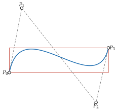
The convex hull of the control points contains a curve (Convex hull) but can be far larger than it. bounding_box returns the box of Axis-aligned bounding box for the curve itself (The tight bounding box of a cubic.). Its candidates come from the roots of the derivative of each coordinate.

Proposition · Bounding box of a cubic

Let \(B\) be the cubic with control points \(P_0, \ldots, P_3 \in \mathbb{R}^d\), and put

\[ a = -P_0 + 3P_1 - 3P_2 + P_3, \quad b = 3P_0 - 6P_1 + 3P_2, \quad c = 3(P_1 - P_0). \]

Then \(B(t) = a t^3 + b t^2 + c t + P_0\). For each coordinate \(k\) let \(T_k\) consist of \(0\), \(1\) and the roots in \((0, 1)\) of

\[ B'_k (t) = 3a_k t^2 + 2 b_k t + c_k \]

when this polynomial is not identically zero; when it is, \(T_k = \lbrace 0, 1\rbrace\). Then the coordinates of the bounding box of \(B([0, 1])\) are

\[ \alpha_k = \min_{t \in T_k} B_k (t), \quad \beta_k = \max_{t \in T_k} B_k (t). \]

CubicBezierSegment.bounding_box

(low, high): two points holding the per-axis minimum and maximum of the curve, found by evaluating it at the candidate parameters of Bounding box of a cubic.

The tight bounding box of a cubic.

Degree elevation

Degree elevation (Degree elevation) writes a curve of degree \(n\) as a curve of degree \(n + 1\) with the same parameterization. The package needs it to write lines and quadratics as cubics, so that every renderer receives four control points. Applying Degree elevation once or twice gives the controls below.

Proposition · Lines and quadratics as cubics

The line from \(P_0\) to \(P_3\), parameterized by \((1 - t) P_0 + t P_3\), is the cubic with controls

\[ P_0, \quad P_0 + 1/3 (P_3 - P_0), \quad P_0 + 2/3 (P_3 - P_0), \quad P_3. \]

The quadratic with controls \(P_0, C, P_3\) is the cubic with controls

\[ P_0, \quad P_0 + 2/3 (C - P_0), \quad P_3 + 2/3 (C - P_3), \quad P_3. \]

In both cases the curve and its parameterization are unchanged.

to_cubic(curve)

In bezierkit.bezier. Turns a linear, quadratic or cubic BezierCurve into a CubicBezierSegment by Lines and quadratics as cubics (a segment is returned as is); higher degrees raise DegreeError.

line_to_cubic(p0, p3)

The cubic of the line from p0 to p3.

quadratic_to_cubic(
    p0,
    control,
    p3
)

The cubic of the quadratic with the given controls.

from bezierkit.bezier import to_cubic

q = BezierCurve.quadratic(Point(0, 0), Point(3, 6), Point(9, 0))
print(to_cubic(q).control_points)
# (Point(coords=(0.0, 0.0)), Point(coords=(2.0, 4.0)),
#  Point(coords=(5.0, 4.0)), Point(coords=(9.0, 0.0)))

Piecewise paths

PiecewiseBezier(
    segments,
    *,
    closed=False,
    continuity_tolerance=1e-9
)
PiecewiseBezier.compound(paths)

segments

The segments in order.

control_points

Their control points.

subpaths

The BezierSubpaths.

at(t)

Evaluate under the uniform parameterization.

at_many(values)

Evaluate at many parameters.

split(t)

Divide the path at t; a parameter inside a segment splits that segment (Subdivision).

segment(t0, t1)

Keep the part between two parameters.

reversed()

Reverse the order of the segments and each segment.

closed

Closure flag.

is_compound

Whether there are several subpaths.

dimension

The dimension \(d\).

A path of cubic segments. Consecutive segments must meet: each segment's p3 must lie within continuity_tolerance of the next one's p0, and a closed path's last p3 within it of the first p0; otherwise ValueError is raised. closed is metadata for exporters (SVG Z, TikZ cycle): it never adds a closing segment.

The package parameterizes a path uniformly. This is a convention of the package, not a standard notion: a path of \(m\) segments \(S_0, \ldots, S_{m-1}\) is the map

\[ P(t) = S_k (m t - k), \quad k = \min(\left\lfloor m t \right\rfloor, m - 1), \quad t \in [0, 1]. \]

Each segment takes an equal share \(1 / m\) of \([0, 1]\), regardless of its length.

from bezierkit import CubicBezierSegment, PiecewiseBezier

path = PiecewiseBezier(
    [
        CubicBezierSegment.from_line(Point(0, 0), Point(2, 0)),
        CubicBezierSegment.from_line(Point(2, 0), Point(2, 4)),
    ]
)
# Point(coords=(2.0, 2.0))
print(path.at(0.75))
# Point(coords=(2.0, 2.0))
print(path.segment(0.25, 0.75).at(1.0))

compound() gathers several paths into one, keeping their subpaths separate, as for a shape with a hole. A compound path has no single parameterization: evaluating, splitting or restricting it raises ValueError; reversal and export work. Splitting or restricting a closed path also raises, except for the whole path or a single point, since a closed path has no first and last point to keep.

Continuity

Two curves meet at a join. Let \(h_S, h_T > 0\), let \(S : [u_0 - h_S, u_0] \to \mathbb{R}^d\) and \(T : [u_0, u_0 + h_T] \to \mathbb{R}^d\) be continuously differentiable as often as needed (with one-sided derivatives at the ends of their intervals), and let \(C\) be the curve that equals \(S\) on the first interval and \(T\) on the second.

Definition · Parametric continuity

For \(k \ge 0\), the curve \(C\) is \(C^k\) at \(u_0\) if \(S^{(j)}(u_0) = T^{(j)}(u_0)\) for \(j = 0, \ldots, k\).

Definition · Geometric continuity \(G^1\)

The curve \(C\) is \(G^1\) at \(u_0\) if \(S(u_0) = T(u_0)\), the tangent vectors \(S'(u_0)\) and \(T'(u_0)\) are non-zero, and \(T'(u_0) = \lambda S'(u_0)\) for some \(\lambda > 0\); that is, the two unit tangents agree.

Parametric and geometric continuity are the standard notions for joined curves Farin (2002)Prautzsch (2002); the geometric notion of every order \(k\) is treated by Barsky (1989). This manual uses \(C^0\), \(C^1\) and \(G^1\) only. A \(C^1\) join with non-zero tangents is \(G^1\).

Proposition · Continuity of cubic joins

Let \(S\) and \(T\) be the cubics with controls \(P_0, \ldots, P_3\) and \(Q_0, \ldots, Q_3\), evaluated at \((u - u_0 + h_S) / h_S\) and \((u - u_0) / h_T\) respectively. + \(C\) is \(C^0\) at \(u_0\) if and only if \(P_3 = Q_0\). + If \(P_3 = Q_0\), then \(C\) is \(C^1\) at \(u_0\) if and only if

\[ (P_3 - P_2) / h_S = (Q_1 - Q_0) / h_T. \]

If \(P_3 = Q_0\), \(P_3 \ne P_2\) and \(Q_1 \ne Q_0\), then \(C\) is \(G^1\) at \(u_0\) if and only if \(Q_1 - Q_0 = \mu (P_3 - P_2)\) for some \(\mu > 0\).
Under the uniform parameterization of PiecewiseBezier, \(h_S = h_T\), so the condition in 2 reads \(P_3 - P_2 = Q_1 - Q_0\).

PiecewiseBezier enforces only \(C^0\), a shared endpoint. Whether a join should also be smooth is the caller's decision: a kink in an indifference curve or a corner in a polyline is meant to stay.