Discrete markets
A discrete market lists units one at a time: each buyer's willingness to pay for one more unit, and each seller's cost of one more unit. Demand and supply are step functions; the equilibrium is a whole number of units, supported by a range of prices.
Schedules
DiscreteDemand(values)
DiscreteSupply(values)Units bought or sold at price; a buyer or seller indifferent at the price trades.
Number of units in the schedule.
Merge several individual schedules into a market schedule (Market curves from individuals).
A demand schedule holds marginal willingness-to-pay values, weakly
decreasing from the first unit to the last; a supply schedule holds
marginal costs, weakly increasing. Values out of order raise
DiscreteMarketError.
Equilibrium
solve_discrete_equilibrium(
    demand,
    supply,
    *,
    price_rule="midpoint"
)Units traded.
Lower end of the supporting price interval.
Upper end of the supporting price interval.
The price chosen from the interval by price_rule.
MIDPOINT (default), LOWER or UPPER; the strings "midpoint", "lower" and "upper" work too.
Values of the traded units.
Costs of the traded units.
Value minus cost of each traded unit.
Whether the interval is a single price.
Trade every unit whose value is at least its cost, and find the interval of prices at which exactly that many units are bought and sold. The result has these fields:
solve_discrete_market(demand_values, supply_values) builds both schedules
from plain tuples and solves in one call. The demand values must descend
and the supply values ascend so that units pair up in order.
from principle_viz import (
    DiscreteDemand,
    DiscreteSupply,
    solve_discrete_equilibrium,
)

demand = DiscreteDemand((11, 9, 7, 5, 3))
supply = DiscreteSupply((1, 3, 5, 8, 10))
eq = solve_discrete_equilibrium(demand, supply)
print(eq.q_star, eq.price_low, eq.price_high, eq.price)
# 3 5.0 7.0 6.0
print(eq.gains_from_trade)
# (10.0, 6.0, 2.0)
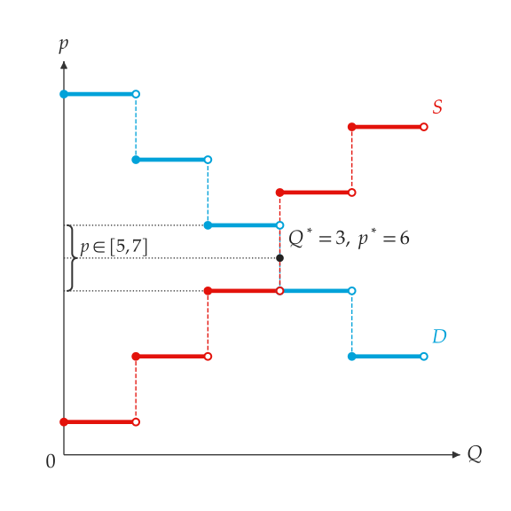
Three units trade at a price interval of 5 to 7, and the midpoint rule reports 6. The gains from trade total \(10 + 6 + 2 = 18\).
compute_discrete_surplus(result)Consumer and producer surplus at the chosen price, in total and unit by
unit (consumer_surplus_by_unit, producer_surplus_by_unit). In the
example above, both are \(5 + 3 + 1 = 9\) at a price of 6.
Figure
MarketFigure.add_discrete_curves(
    demand=None,
    supply=None,
    *,
    demand_label="$D$",
    supply_label="$S$"
)
MarketFigure.add_discrete_equilibrium(result)
Draw each unit as a step \([q, q + 1)\): a filled point where the step starts (included) and an open point where it ends (excluded), joined to the next step by a dashed riser. Pass one schedule or both. The equilibrium marks \(Q^*\) and the price interval on the axes.
fig = MarketFigure(
    x_max=5.5,
    y_max=12,
    title="Discrete Demand and Supply",
)
fig.add_discrete_curves(demand, supply)
fig.add_discrete_equilibrium(eq)
fig.finalize()
The figure for this example is shown in Discrete demand and supply..