Elasticity and total revenue

Price elasticity

compute_point_elasticity(demand, quantity)
compute_arc_elasticity(
    q0,
    p0,
    q1,
    p1
)

The point price elasticity of a line at a quantity,

\[ \epsilon = (\mathrm{d} Q) / (\mathrm{d} p) \cdot p / Q, \]

and the arc (midpoint) elasticity between two points,

\[ \epsilon = (\Delta Q / \overline{Q}) / (\Delta p / \overline{p}), \]

where \(\overline{Q}\) and \(\overline{p}\) are the averages of the two points. Both are negative for a downward-sloping demand.

from principle_viz import (
    compute_arc_elasticity,
    compute_point_elasticity,
    line_from_inverse,
)

demand = line_from_inverse(10.0, -1.0)
# -1.5
print(compute_point_elasticity(demand, 4))
# -1.0 (unit elastic)
print(compute_point_elasticity(demand, 5))
# -1.0
print(compute_arc_elasticity(4, 6, 6, 4))

At \(Q = 4\) the elasticity is \(-1.5\), so demand is elastic. \(Q = 5\) is unit elastic, the midpoint of \(p = 10 - Q\). The arc elasticity uses the averages of the two points, so \((4, 6)\) to \((6, 4)\) and the reverse give the same value.

classify_elasticity(value) in principle_viz.core.elasticity names the absolute value: "elastic" above 1, "unit_elastic" at 1 and "inelastic" below 1.

Total revenue

elasticity_revenue_schedule(
    demand,
    *,
    samples=101
)

points

RevenuePoints with quantity, price, total_revenue, elasticity and classification.

unit_elastic_quantity

Quantity at the midpoint of the line.

unit_elastic_price

Price at the midpoint of the line.

maximum_revenue

Total revenue at that point.

choke_quantity

The quantity-axis intercept.

choke_price

The price-axis intercept.

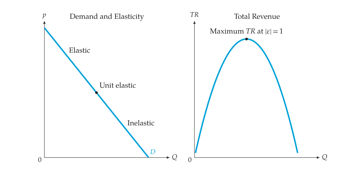
Sample a linear demand from \(Q = 0\) to its choke quantity and return, at each point, price, total revenue \(p Q\), elasticity and its class. Total revenue peaks where demand is unit elastic, at the midpoint of the line.

For \(p = 12 - Q\), maximum revenue is 36 at \(Q = 6\), \(p = 6\).

elasticity_revenue_canvases(
    demand,
    result,
    *,
    theme=None,
    labels=None,
    visibility=None
)

Two mosaickit canvases, in principle_viz.visuals.revenue: the demand curve, labelled "Elastic", "Unit elastic" and "Inelastic" along its length with the unit-elastic point marked, and total revenue against quantity with its maximum marked. Each canvas carries its own title. Place them side by side with mosaickit.CanvasGrid (see Elasticity along demand and total revenue.).

from mosaickit import CanvasGrid
from principle_viz import PlotTheme, elasticity_revenue_schedule
from principle_viz.visuals.revenue import (
    elasticity_revenue_canvases,
)

demand = line_from_inverse(12.0, -1.0)
schedule = elasticity_revenue_schedule(demand)
canvases = elasticity_revenue_canvases(
    demand,
    schedule,
    theme=PlotTheme(),
)
CanvasGrid(canvases, rows=1).save(
    "elasticity_total_revenue.png"
)

The output is shown in Elasticity along demand and total revenue..

Comments