Market failures

Externalities

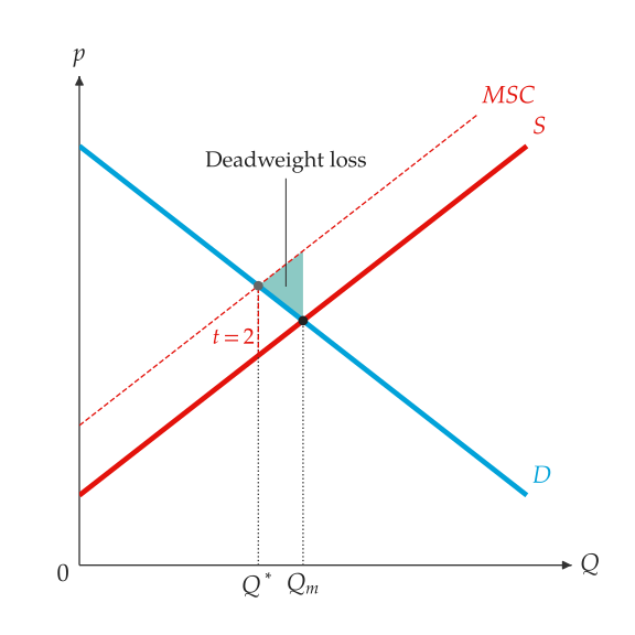
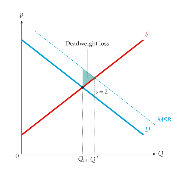
When production imposes a cost on third parties, or consumption confers a benefit on them, the market quantity differs from the social optimum. A Pigouvian tax or subsidy equal to the external effect at the optimum restores the optimal quantity Pigou (1920).

ExternalityScenario(
    marginal_external_cost=0.0,
    marginal_external_benefit=0.0
)

A constant marginal external cost, which adds to supply to give the marginal social cost, and/or a marginal external benefit, which adds to demand to give the marginal social benefit. Both must be non-negative.

analyze_externality(
    demand,
    supply,
    scenario
)

The private and social outcomes: private_equilibrium, social_equilibrium, social_demand, social_supply, corrective_tax, corrective_subsidy, quantity_distortion and deadweight_loss.

from principle_viz import (
    ExternalityScenario,
    analyze_externality,
)

demand = line_from_inverse(12.0, -1.0)
scenario = ExternalityScenario(marginal_external_cost=2)
result = analyze_externality(demand, supply, scenario)
print(
    result.private_equilibrium.q_star,
    result.social_equilibrium.q_star,
)
# 5.0 4.0
print(result.corrective_tax, result.deadweight_loss)
# 2.0 1.0

MarketFigure.add_externality(result)

Draw the social curve, mark \(Q_m\) (market) and \(Q^*\) (optimum) on the quantity axis, label the corrective tax \(t\) or subsidy \(s\) across the gap at \(Q^*\), and shade the deadweight loss (see A negative externality. and A positive externality.).

Common resources

analyze_common_resource(
    benefit,
    cost,
    *,
    marginal_congestion_cost
)

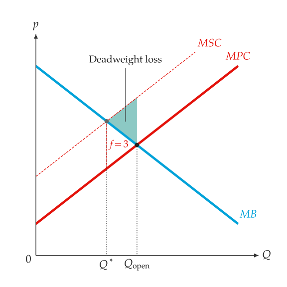
Treat congestion or depletion as a marginal external cost: open access uses the resource until marginal benefit equals private cost, beyond the efficient level Hardin (1968). The result has open_access_equilibrium, efficient_equilibrium, social_cost, overuse, corrective_fee and deadweight_loss.

With \(M B = 12 - Q\), \(M P C = 2 + Q\) and a congestion cost of 3, open access uses 5 units, the efficient level is 3.5 and corrective_fee is 3.

MarketFigure.add_common_resource(result)

Draw the social cost, mark \(Q^*\) and \(Q_\text{open}\), and shade the deadweight loss. Name the curves \(M B\) and \(M P C\) in add_curves(). See Overuse of a common resource..

Public goods

IndividualBenefit(name, marginal_benefit)
analyze_public_good(
    individuals,
    cost,
    *,
    samples=101
)

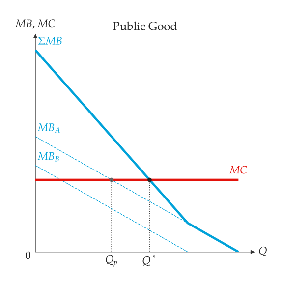
Everyone consumes the whole quantity of a public good, so marginal benefits add vertically. The efficient quantity sets their sum equal to marginal cost Samuelson (1954); private provision stops where the highest individual benefit meets marginal cost. The result has efficient_quantity, efficient_marginal_value, private_provision_quantity, free_rider_gap and the sampled points.

from principle_viz import IndividualBenefit, analyze_public_good

result = analyze_public_good(
    (
        IndividualBenefit("$MB_A$", line_from_inverse(8, -1)),
        IndividualBenefit("$MB_B$", line_from_inverse(6, -1)),
    ),
    # constant marginal cost of 5
    line_from_inverse(5, 0),
)
print(
    result.efficient_quantity, result.private_provision_quantity
)
# 4.5 3.0

public_good_canvas(
    result,
    *,
    theme=None,
    labels=None,
    visibility=None
)

A mosaickit canvas, in principle_viz.visuals.market_failures, with each marginal benefit, their vertical sum, marginal cost, and \(Q_p\) and \(Q^*\) on the quantity axis (see The vertical sum of marginal benefits.).

Comments