Market curves from individuals

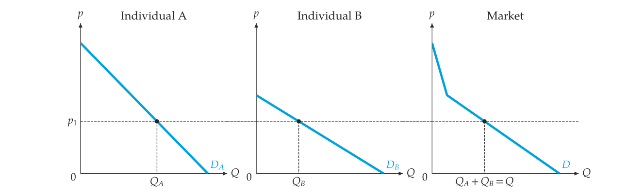
A market curve is the horizontal sum of the individual curves: at each price, market quantity is the sum of the quantities every buyer (or seller) chooses at that price. A buyer buys nothing above the choke price and a seller sells nothing below the minimum price. The market curve of linear individuals is piecewise linear, with a kink where each additional individual enters.

Summing linear curves

market_demand(individuals)
market_supply(
    individuals,
    *,
    p_max
)

Sum downward-sloping (demand) or upward-sloping (supply) individual lines. The supply sum runs from the lowest minimum price up to p_max. Curves of the wrong slope raise AggregationError.

PiecewiseLinear(points)

q_at(p)

Quantity at a price; a price outside the curve raises PiecewiseLinearError.

p_at(q)

Price at a quantity; a quantity outside the curve raises PiecewiseLinearError.

points

All vertices.

kinks

The interior vertices where the slope changes.

domain

Quantity range covered.

price_range

Price range covered.

breakpoints()

Vertex prices in ascending order.

integrate_q()

Area under \(Q(p)\) between the prices p_low and p_high.

A demand or supply curve through points \((Q, p)\), ordered by quantity. If the first point has \(Q = 0\), quantity is zero at prices beyond it.

from principle_viz import (
    line_from_inverse,
    market_demand,
    market_supply,
)

# p = 10 - 2Q
a = line_from_inverse(10, -2)
# p = 6 - 0.5Q
b = line_from_inverse(6, -0.5)
demand = market_demand((a, b))
# ((0.0, 10.0), (2.0, 6.0), (17.0, 0.0))
print(demand.points)
# 7.0 = Q_A + Q_B = 3 + 4
print(demand.q_at(4))

Buyer B enters at a price of 6, giving the kink \((2, 6)\). At a price of 4, \(Q_A = 3\) and \(Q_B = 4\), so market demand is 7.

solve_piecewise_equilibrium(demand, supply)
piecewise_surplus(
    demand,
    supply,
    result
)

The exact market equilibrium, solved segment by segment, and the consumer and producer surplus at it, integrated along price.

from principle_viz import (
    piecewise_surplus,
    solve_piecewise_equilibrium,
)

c = line_from_inverse(2, 1)
d = line_from_inverse(5, 0.5)
supply = market_supply((c, d), p_max=10)
eq = solve_piecewise_equilibrium(demand, supply)
# 3.818 5.273
print(round(eq.q_star, 3), round(eq.p_star, 3))
cs, ps = piecewise_surplus(demand, supply, eq)

piecewise_surplus() returns the consumer and producer surplus integrated along price.

Summing discrete schedules

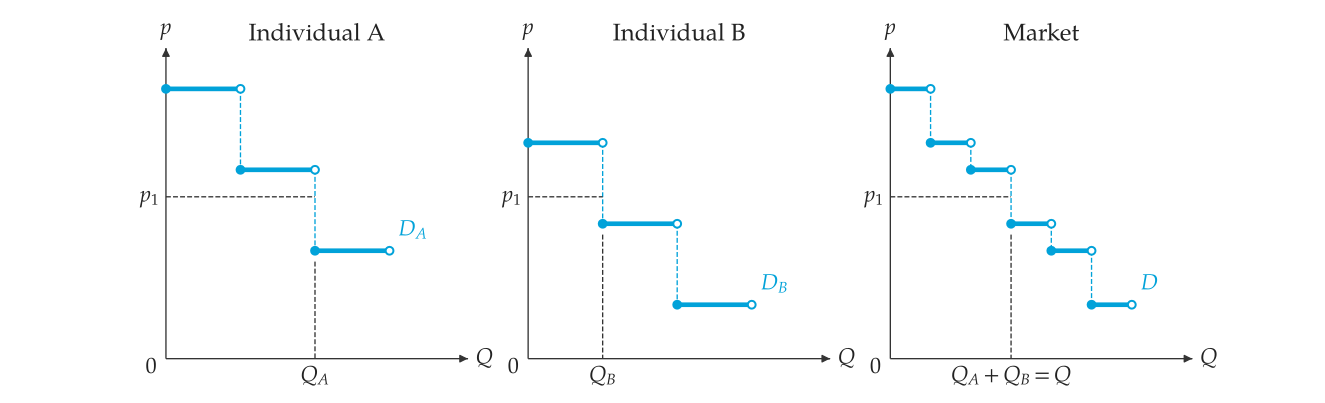
DiscreteDemand.combine(*schedules) merges every buyer's reservation prices into one market schedule, highest first; DiscreteSupply.combine() merges unit costs, lowest first. Equal values remain separate units, and the result works with solve_discrete_equilibrium() (Discrete markets). The output is shown in Combining two discrete demand schedules..

from principle_viz import DiscreteDemand

first = DiscreteDemand((10, 7, 4))
second = DiscreteDemand((8, 5, 2))
market = DiscreteDemand.combine(first, second)
print(market.values)
# (10.0, 8.0, 7.0, 5.0, 4.0, 2.0)

Aggregation figures

demand_aggregation_figure(
    individuals,
    *,
    price,
    price_label="$p_1$",
    link_price=False,
    ...
)
supply_aggregation_figure(
    individuals,
    *,
    price,
    p_max,
    ...
)
discrete_demand_aggregation_figure(
    individuals,
    *,
    price,
    ...
)
discrete_supply_aggregation_figure(
    individuals,
    *,
    price,
    ...
)

link_priceboolDefault: False

Run the price line across every panel and the gaps between them, marking the price on the first panel only.

theme

As for MarketFigure (Palettes and themes).

palette

As for MarketFigure (Palettes and themes).

labels

Label overrides by layer id (Labels and layers).

visibility

Layer visibility by layer id (Labels and layers).

One panel per individual, then the market, side by side and sharing the price axis. individuals maps each name to a curve or schedule; the curves are named \(D_A\), \(D_B\), ... and \(D\) (or \(S_A\), ..., \(S\)). Dashed guides at price mark \(Q_A\), \(Q_B\) and \(Q_A + Q_B = Q\). supply_aggregation_figure() also needs p_max.

The returned AggregationFigure has save(), hide(), show(), configure_label(), layer_ids and label_ids, like MarketFigure.

from principle_viz import demand_aggregation_figure

fig = demand_aggregation_figure(
    {"A": a, "B": b},
    price=4,
    link_price=True,
)
fig.save("market_demand.png")

The output of demand_aggregation_figure() is shown in Market demand as the horizontal sum..

Comments