Fitting

Fitting turns a smooth function or a list of sampled points into a PiecewiseBezier whose error is measured and reported, segment by segment, in the coordinate units of the curve. The functions live in bezierkit.fitting.

Adaptive Hermite fitting

The fit of a parametric curve \(C : [t_0, t_1] \to \mathbb{R}^d\) on an interval \([a, b]\) is the cubic Hermite interpolant of Cubic Hermite interpolant, taken for each coordinate (Hermite interpolation). The package measures its error at \(q\) equally spaced probe parameters \(\tau_j = a + j (b - a) / (q - 1)\), \(j = 0, \ldots, q - 1\), where \(q\) is error_samples:

\[ e = \max_{0 \le j \le q-1} \left\lVert C(\tau_j) - H(\tau_j) \right\rVert_2. \]

This measured error is a convention of the package; it is never larger than the true maximum error of the segment.

fit_parametric(
    function,
    derivative,
    *,
    t0,
    t1,
    tolerance,
    max_depth=20,
    max_segments=4096,
    error_samples=9
)

tolerancefloat

Allowed error, in coordinate units; must be positive.

max_depthintDefault: 20

Largest number of halvings of the starting interval.

max_segmentsintDefault: 4096

Largest number of segments in the result.

error_samplesintDefault: 9

Probe parameters per segment, at least 3.

Fit a parametric curve \(C(t)\), given as a function returning Points and its derivative returning Vectors, over \([t_0, t_1]\). The algorithm is a recursive bisection:

• Build the Hermite segment on the current interval from \(C\) and \(C'\) at its ends (Hermite interpolation).
• Measure its error \(e\).
• If \(e\) is at most tolerance, keep the segment, recording \(e\) as its fit_error. Otherwise halve the interval and fit each half.

Every accepted segment therefore meets the tolerance at its probe parameters. If an interval still fails at depth max_depth, or keeping it would exceed max_segments, ToleranceNotMet is raised rather than a worse path returned.

fit_graph(
    function,
    derivative,
    *,
    x0,
    x1,
    tolerance,
    ...
)

Fit the graph \(y = f(x)\) for \(x \in [x_0, x_1]\): fit_parametric with \(C(x) = (x, f(x))\) and \(C'(x) = (1, f'(x))\), the same options, and the error measured as a Euclidean distance in the \((x, y)\) plane.

from bezierkit.fitting import fit_graph

path = fit_graph(
    lambda x: 4 / x**2,
    lambda x: -8 / x**3,
    x0=0.8,
    x1=3,
    tolerance=1e-3,
)
# 10
print(len(path.segments))
# 0.000676
print(max(s.fit_error for s in path))

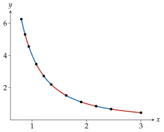
Segments are short where the curve bends sharply and long where it is nearly straight (Adaptive fit of \(4 / x^2\); segments alternate colour.). The Hermite error bound predicts how deep the bisection has to go:

Corollary · Depth of adaptive fitting

Let each coordinate of \(C\) be four times continuously differentiable on \([t_0, t_1]\) with \(|C_k^{(4)}| \le M\), put \(L = |t_1 - t_0|\), and let \(d\) be the dimension and \(\epsilon > 0\) the tolerance. Put

\[ k^* = \max(0, \left\lceil 1/4 \log_2 (\sqrt\lbrace d\rbrace M L^4 / (384 \epsilon)) \right\rceil), \]

with \(k^* = 0\) when \(M = 0\). Every interval at a depth \(k \ge k^*\) passes the error test. Hence if max_depth \(\ge k^*\) and max_segments \(\ge 2^{k^*}\), fit_parametric does not raise ToleranceNotMet, and no interval deeper than \(k^*\) is created.

The measured error is a lower bound for the true maximum error of a segment: it is checked only at the probe parameters. Increase error_samples when the curve could wiggle between them.

Polyline simplification

Definition · Distance to a segment

For \(x, a, b \in \mathbb{R}^d\), the distance from \(x\) to the segment \([a, b]\) is

\[ \text{dist}(x, [a, b]) = \min_{\lambda \in [0, 1]} \left\lVert x - a - \lambda (b - a) \right\rVert_2. \]

Polyline simplification by recursive subdivision is the Ramer--Douglas--Peucker algorithm Ramer (1972)Douglas (1973). fit_polyline uses the distance of Distance to a segment throughout.

fit_polyline(
    points,
    *,
    tolerance,
    closed=False,
    duplicate_tolerance=1e-12,
    preserve_corners=True,
    corner_angle=pi/4
)

Simplify sampled points into a path of straight chords, each written as an exact cubic (Lines and quadratics as cubics). The steps are:

• Drop each point within duplicate_tolerance of the one kept before it. A closed polyline also drops a final copy of its first point, and is rotated so that it starts at its lexicographically smallest point, which makes the output independent of where the samples began.
• Keep the end points and, with preserve_corners, every vertex where the direction turns by at least corner_angle radians.
• Between consecutive kept vertices, apply the recursive step: if the vertex farthest from the chord is within tolerance of it, the chord replaces the whole run; otherwise keep that vertex and recurse on both sides.

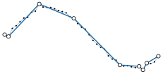
Each chord's fit_error is the largest distance from the vertices it replaced to the chord (41 noisy samples simplified with tolerance \(0.08\).).

The recursion makes at most as many levels as there are vertices and scans each vertex once per level, so it is quadratic in the number of vertices in the worst case. Hershberger (1994) give an \(O(n \log n)\) implementation of the algorithm.

Proposition · Polyline tolerance

Let \(v_0, \ldots, v_N\) be the vertices left by step 1 (for a closed polyline \(v_N = v_0\)), let \(0 = a_0 < \ldots < a_m = N\) be the indices of the vertices that the output keeps, and let \(\epsilon\) be tolerance. For every \(j\) and every \(i\) with \(a_j \le i \le a_{j+1}\),

\[ \text{dist}(v_i, [v_{a_j}, v_{a_{j+1}}]) \le \epsilon. \]

In particular the fit_error of every output segment is at most \(\epsilon\).

Corollary · Deviation from the polyline

With the notation of Polyline tolerance: + Every point of the polyline \(v_0 v_1 \ldots v_N\) lies within \(\epsilon\) of one chord \([v_{a_j}, v_{a_{j+1}}]\) of the output. + Every input point lies within \(\epsilon + \delta\) of a chord, where \(\delta\) is duplicate_tolerance; the points left by step 1 lie within \(\epsilon\).

maximum_polyline_deviation(points, path)

The largest distance from any of the points to the nearest chord \(P_0 P_3\) of the path's segments: a check of Polyline tolerance and Deviation from the polyline that also covers the points step 1 dropped.

Like any method that sees only samples, fit_polyline bounds the deviation from the samples, not from an unknown continuous curve between them; sample more densely for a closer match.

Comments