Welfare
Welfare analysis compares a market outcome with its alternatives: consumer surplus, producer surplus, government revenue and deadweight loss.
Market outcomes
MarketOutcome(
    quantity,
    consumer_price,
    producer_price,
    label=""
)A free market: both prices are \(p^*\).
After a tax (Taxes and subsidies).
After a subsidy.
Under a price ceiling or floor (Price controls).
A quantity with the price buyers pay and the price sellers receive. The
two prices differ under a tax or a subsidy; the gap times the quantity is
government revenue (negative for a subsidy). It lives in
principle_viz.welfare.surplus, together with constructors from each
kind of result:
Surplus
compute_surplus(
    demand,
    supply,
    outcome,
    baseline_outcome=None
)Area between demand and the consumer price.
Area between the producer price and supply.
Government revenue (negative for a subsidy).
The sum of the three.
Surplus lost relative to the baseline.
The corner points of each area, used to draw them.
The welfare decomposition at outcome. With a baseline_outcome, the
deadweight loss is measured against it. The SurplusResult has these
fields:
from principle_viz import compute_surplus, solve_equilibrium
from principle_viz.welfare.surplus import (
    outcome_from_equilibrium,
)

eq = solve_equilibrium(demand, supply)
outcome = outcome_from_equilibrium(eq)
surplus = compute_surplus(demand, supply, outcome)
# 8.0 8.0
print(surplus.consumer_surplus, surplus.producer_surplus)
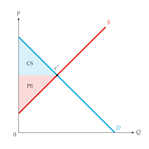
\((10 - 6) \times 4 / 2 = (6 - 2) \times 4 / 2 = 8\); the free market has no deadweight loss.
compare_surplus(
    demand,
    supply,
    baseline_outcome,
    policy_outcome
)
Both decompositions and the changes between them: baseline, policy,
delta_consumer_surplus, delta_producer_surplus, delta_tax_revenue,
delta_total_surplus and deadweight_loss. Taxes and subsidies uses it for a
tax.
Figures
MarketFigure.add_welfare(
    result,
    *,
    labels=True,
    regions=None
)False shades the regions without naming them.
Limit the shading to some of "cs", "ps", "tax_revenue" and "dwl".
Shade consumer surplus, producer surplus, tax revenue and deadweight loss, and name each region: inside it when the name fits, by its short name (CS, PS, Tax, DWL) when only that fits, otherwise by a callout that covers no line, point or other text.
fig = MarketFigure(x_max=12, y_max=12)
fig.add_curves(demand, supply, q_max=10)
fig.add_welfare(surplus)
fig.add_equilibrium(eq)
fig.finalize()
The output is shown in Consumer and producer surplus at equilibrium..
MarketFigure.add_welfare_transition(
    *,
    baseline_outcome,
    policy_outcome,
    surplus
)
The same regions together with guide lines at the baseline and policy quantities and prices, for comparing before and after.
Deadweight-loss reports
build_dwl_report(rows)Turn (name, baseline, policy) triples of SurplusResults into report
rows (DWLScenarioRow) with the change in quantity, in each surplus and
the deadweight loss. save_dwl_report_csv() and save_dwl_report_json()
in principle_viz.welfare.report write them to a file.