Derivatives, reversal and subdivision

Each operation acts on the control points alone and returns a new curve that keeps the evaluator of the original.

Derivatives

The derivative \(B'(t)\) of a Bézier curve is the derivative of its coordinate functions, which are polynomials in \(t\); it is a vector in \(\mathbb{R}^d\).

Lemma · Derivative of the Bernstein polynomials

For \(n \ge 1\) and every integer \(i\),

\[ b'_{i,n}(t) = n [b_{i-1,n-1}(t) - b_{i,n-1}(t)]. \]

This is Lemma 1.4 of Floater (2025).

Theorem · Hodograph

The derivative of a degree-\(n\) Bézier curve (\(n \ge 1\)) is the degree \(n - 1\) Bézier curve

\[ B'(t) = \sum_{i=0}^{n-1} b_{i,n-1}(t) \cdot n (P_{i+1} - P_i). \]

The curve of control points \(n(P_{i+1} - P_i)\) is the hodograph of \(B\) (Theorem 1.8 of Floater (2025); see also Farin (2002)).

Corollary · End tangents

\(B'(0) = n(P_1 - P_0)\) and \(B'(1) = n(P_n - P_{n-1})\).

This is why a curve leaves \(P_0\) in the direction of \(P_1\) and arrives at \(P_n\) from \(P_{n-1}\).

BezierCurve.derivative(order=1)

The order-th derivative as a BezierCurve, by applying Hodograph order times. The derivative of a constant (degree 0) is the zero curve of degree 0; order=0 returns the curve itself.

d = curve.derivative()
print(list(d.control_points))
# [Point(coords=(3.0, 6.0)), Point(coords=(6.0, 0.0)), Point(coords=(3.0, -6.0))]
# Point(coords=(4.5, 0.0)): the tangent at the top is horizontal
print(d.at(0.5))

Reversal

Lemma · Symmetry

\(b_{i,n}(1 - t) = b_{n-i,n}(t)\) for all \(i\) and \(t\).

Proposition · Reversal

The curve with control points \(P_n, \ldots, P_0\) is \(t |\to B(1 - t)\).

BezierCurve.reversed

The curve traced in the opposite direction, by Reversal.

Subdivision

Running de Casteljau's algorithm at \(t = c\) does more than evaluate: the first points of each round form the control polygon of the part of the curve before \(c\), and the last points that of the part after it (Splitting the cubic at \(t = 0.4\).).

Theorem · Subdivision

Let \(c \in [0, 1]\), and compute the de Casteljau points of de Casteljau points at \(t = c\). Put \(L_j = P_0^{(j)}\) and \(R_j = P_j^{(n-j)}\) for \(j = 0, \ldots, n\). Then for every \(s \in [0, 1]\)

\[ B(c s) = \sum_{j=0}^n b_{j,n}(s) L_j \]

and

\[ B(c + (1 - c) s) = \sum_{j=0}^n b_{j,n}(s) R_j. \]

The result is classical; see Floater (2025) (Section 8.4, where it is derived from the blossom) and Farin (2002).

BezierCurve.split(float)
BezierCurve.segment(t0, t1)

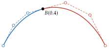
split(c) returns the two curves of Subdivision, each of the same degree and parameterized over \([0, 1]\). segment(t0, t1) returns the part of the curve between \(t_0\) and \(t_1\), reparameterized over \([0, 1]\); when \(t_0 = t_1\) it is the single point \(B(t_0)\), a curve of degree 0. Parameters outside \([0, 1]\), or \(t_0 > t_1\), raise.

segment() splits twice: first at \(t_1\), keeping the left part, then that part at \(t_0 / t_1\), keeping the right part.

Corollary · Segment extraction

For \(0 \le t_0 < t_1 \le 1\) the curve returned by segment(t0, t1) is \(s |\to B(t_0 + (t_1 - t_0) s)\).

left, right = curve.split(0.4)
# both B(0.4) = (1.552, 1.44)
print(left.at(1.0), right.at(0.0))
# B(0.5) = (2.0, 1.5)
print(curve.segment(0.25, 0.75).at(0.5))

Comments