Advanced Models

Advanced models extend the built-in utility families with user-defined functions, more than two goods, or goods that are inferior or Giffen.

Extensible models

Use these models when a predefined two-good utility class is not enough.

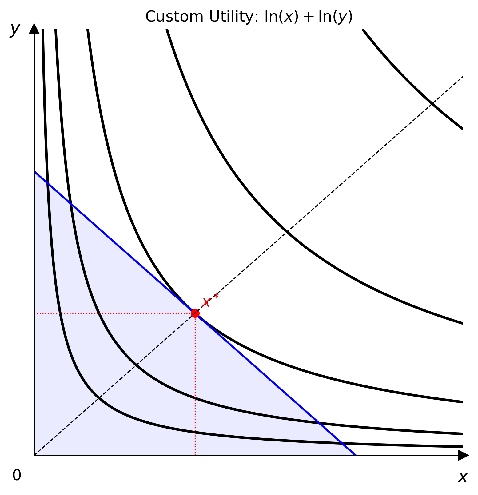
Custom UtilityMulti-Good Cobb-Douglas

CustomUtility wraps any vectorised Python callable as an econ-viz model.

\[ U(x,y)=\ln x+\ln y \]

The equation above is one example. The callable must accept two NumPy arrays and return an array with the same shape.

Parameters

Parameter	Meaning
func	Vectorised utility function of \(x\) and \(y\)
name	Display name for the custom model

Example

import numpy as np
from econ_viz import Canvas, levels, solve
from econ_viz.models import CustomUtility

model = CustomUtility(
    func=lambda x, y: np.log(x) + np.log(y),
    name="log+log",
)
eq = solve(model, px=2.0, py=3.0, income=30.0)

(
    Canvas(x_max=20, y_max=15, title="Custom Utility")
    .add_utility(model, levels=levels.around(eq.utility, n=5))
    .add_budget(2.0, 3.0, 30.0)
    .add_equilibrium(eq)
    .save("custom.png")
)

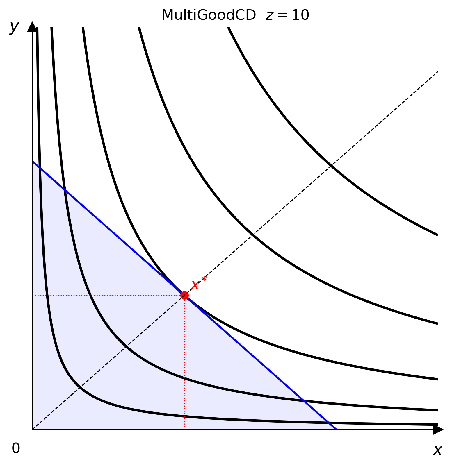
MultiGoodCD represents Cobb-Douglas preferences over \(N\) goods.

\[ U(x_1,\ldots,x_N)=\prod_{i=1}^{N}x_i^{\alpha_i} \]

freeze() fixes every good except \(x\) and \(y\), then returns a CustomUtility that can be drawn on a two-dimensional canvas.

Parameters

Parameter	Meaning
shares	Mapping from each good name to its exponent \(\alpha_i\)
freeze(...)	Fixed quantities for goods other than \(x\) and \(y\)

Example

from econ_viz import Canvas, levels, solve
from econ_viz.models import MultiGoodCD

model = MultiGoodCD({"x": 0.3, "y": 0.3, "z": 0.4})
two_good_model = model.freeze(z=10.0)
eq = solve(two_good_model, px=2.0, py=3.0, income=30.0)

(
    Canvas(x_max=20, y_max=15, title="Multi-Good Cobb-Douglas")
    .add_utility(
        two_good_model,
        levels=levels.around(eq.utility, n=5),
    )
    .add_budget(2.0, 3.0, 30.0, fill=True)
    .add_equilibrium(eq)
    .save("multigood.png")
)

Inferior and Giffen goods

Haagsma implements the utility function of Haagsma(2012), in which good \(x\) is always inferior and becomes a Giffen good when income is high enough.

\[ U(x,y)=\alpha_x\ln(x-\gamma_x)-\alpha_y\ln(\gamma_y-y), \qquad 0<\alpha_x<\alpha_y,\quad x>\gamma_x,\quad 0\le y<\gamma_y \]

At an interior optimum, Marshallian demand for \(x\) has a closed form:

\[ x^*=\frac{\alpha_x(\gamma_y p_y-I)}{(\alpha_y-\alpha_x)\,p_x}+\frac{\alpha_y\gamma_x}{\alpha_y-\alpha_x} \]

so \(\partial x^*/\partial I<0\) for every price and income. The sign of \(\partial x^*/\partial p_x\) depends on income:

Income	Good \(x\)
\(I<\gamma_y p_y\)	Inferior; demand still falls as \(p_x\) rises
\(I=\gamma_y p_y\)	Inferior; substitution and income effects cancel
\(\gamma_y p_y<I<\gamma_y p_y+\gamma_x p_x\)	Giffen; demand rises with \(p_x\)

With \(I\ge\gamma_y p_y+\gamma_x p_x\) the consumer can push \(y\) towards \(\gamma_y\), utility grows without bound, and no optimum exists; solve() raises an error.

Parameters

Parameter	Meaning
alpha_x	Weight \(\alpha_x\) on good \(x\), below alpha_y
alpha_y	Weight \(\alpha_y\) on good \(y\)
gamma_x	Lower bound \(\gamma_x\) of good \(x\)
gamma_y	Upper bound \(\gamma_y\) of good \(y\)

demand(px, py, income) returns the closed-form bundle, and is_giffen(px, py, income) reports whether \(x\) is a Giffen good.

Example

from econ_viz import Canvas, Effect
from econ_viz.models import Haagsma
from econ_viz.optimizer import decompose_price_effect

model = Haagsma(alpha_x=1.0, alpha_y=2.0, gamma_x=2.0, gamma_y=27.0)
model.is_giffen(px=2.0, py=1.0, income=28.0)  # True

result = decompose_price_effect(model, px=(2.0, 1.0), py=1.0, income=28.0, method="hicks")

(
    Canvas(x_max=16, y_max=32, title="Haagsma: Giffen good")
    .add_decomposition(
        result,
        show_x_projections=True,
        substitution=Effect(label="SE"),
        income=Effect(label="IE"),
    )
    .save("haagsma.png")
)

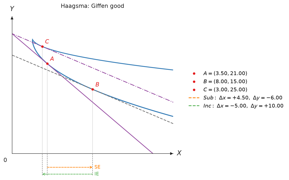
When \(p_x\) falls from 2 to 1, the substitution effect raises \(x\) by 4.5 while the income effect lowers it by 5, so demand for \(x\) falls.

Comments