Canvas

Canvas is the central drawing surface. It manages a single matplotlib figure styled in the convention of microeconomic textbook diagrams: first-quadrant axes, arrow tips, LaTeX-rendered labels, and no numeric tick marks.

Constructor

from econ_viz import ArrowStyle, Axis, Canvas, Stroke, themes

cvs = Canvas(
    x_max=20,
    y_max=15,
    title=r"Cobb-Douglas $x^{0.5} y^{0.5}$",
    dpi=300,
    font="DejaVu Sans",
    math_font="stix",
    axis_stroke=Stroke(width=1.0, arrow=ArrowStyle.TRIANGLE),
    x_axis=Axis(label="x", label_position="right"),  # "top", "right", or "bottom"
    y_axis=Axis(label="y", label_position="top"),    # "left", "top", or "right"
    theme=themes.default,
)

Parameter	Type	Default	Description
`x_max`	float	10	Upper bound of the horizontal axis
`y_max`	float	10	Upper bound of the vertical axis
`x_axis`	`Axis`	None	Label, label position, and stroke of the horizontal axis
`y_axis`	`Axis`	None	Label, label position, and stroke of the vertical axis
`x_label`	str	`"X"`	Shorthand for `Axis(label=...)` on the horizontal axis
`y_label`	str	`"Y"`	Shorthand for `Axis(label=...)` on the vertical axis
`title`	str or None	None	Figure title
`dpi`	int	300	Raster export resolution (clamped to 1–1200)
`x_label_pos`	str or `LabelPosition`	`"right"`	Shorthand for `Axis(label_position=...)`: above, right of, or below the arrow tip
`y_label_pos`	str or `LabelPosition`	`"top"`	Shorthand for `Axis(label_position=...)`: left of, above, or right of the arrow tip
`font`	str or sequence	None	Font family or fallback list for every text element
`math_font`	str	None	Matplotlib math font: `dejavusans`, `dejavuserif`, `cm`, `stix`, or `stixsans`
`axis_stroke`	`Stroke`	theme default	Shared width, style, colour, and arrowhead for both axes
`x_axis_stroke`	`Stroke`	None	Horizontal-axis override, shorthand for `Axis(stroke=...)`
`y_axis_stroke`	`Stroke`	None	Vertical-axis override, shorthand for `Axis(stroke=...)`
`theme`	Theme	`themes.default`	Colour and style theme

When the same setting is given twice, the Axis field wins. For the axis line, the order from highest to lowest is Axis.stroke, x_axis_stroke, axis_stroke, x_line_style / x_arrow_style, and theme.axis_stroke.

Methods

All drawing methods return self, so calls can be chained.

Utility curves

Draws indifference curves for a utility model. Pass an integer to levels for automatically spaced curves, or a list of utility values, such as levels.around(eq.utility, n=5), to place them around the optimum.

cvs.add_utility(
    func,
    levels=3,          # count or list of levels
    stroke=None,       # default: theme.ic_stroke
    ray_stroke=None,
    show_rays=False,
    show_kinks=False,
    kink_radius=1.0,
    show_bliss=True,   # ★ at bliss point (Satiation)
    kink_marker=None,  # default: theme.kink_marker
    bliss_marker=None, # default: theme.bliss_marker
    ic_label=None,     # Label for utility levels at curve ends
    bliss_label=None,  # str or Label
    highlight_level=None, # nearest level becomes the focal curve
    secondary_stroke=None,# style of the remaining curves
    label_style="numeric",# "numeric" or textbook-style "ordinal"
)

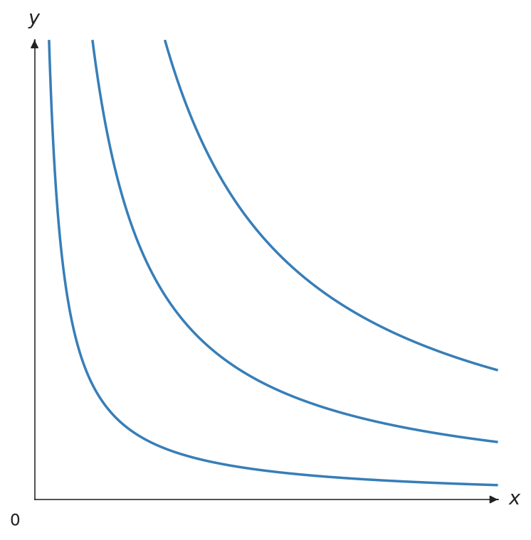
Indifference curves drawn with add_utility

Focal and secondary curves

Pass the equilibrium utility to highlight_level to emphasize the nearest available level without drawing a second contour set yourself. The other levels use theme.secondary_ic_stroke, or an explicit secondary_stroke.

from econ_viz import Canvas, Stroke, levels, solve
from econ_viz.models import CobbDouglas

model = CobbDouglas(0.5, 0.5)
eq = solve(model, px=2, py=3, income=30)
lvls = levels.around(eq.utility, n=5)

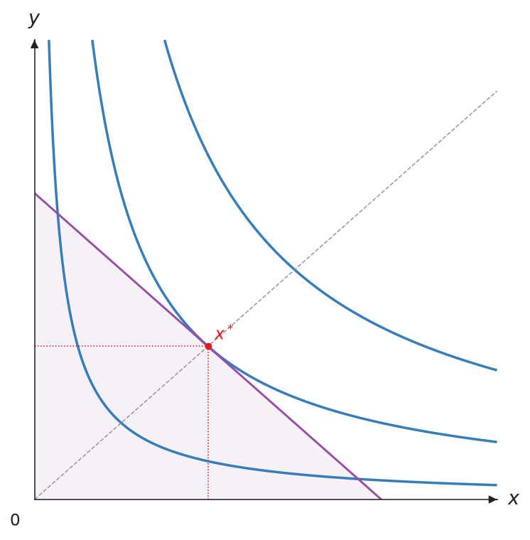
(Canvas(x_max=20, y_max=15)
 .add_utility(
     model,
     levels=lvls,
     highlight_level=eq.utility,
     secondary_stroke=Stroke(width=1, opacity=0.35),
     show_ic_labels=True,
     label_style="ordinal",
 )
 .add_budget(2, 3, 30, fill=True)
 .add_equilibrium(eq))

label_style="numeric" uses the formatted utility values; "ordinal" produces textbook labels \(u_1,u_2,\ldots\). Labels follow the local curve angle and are kept away from the visible boundary.

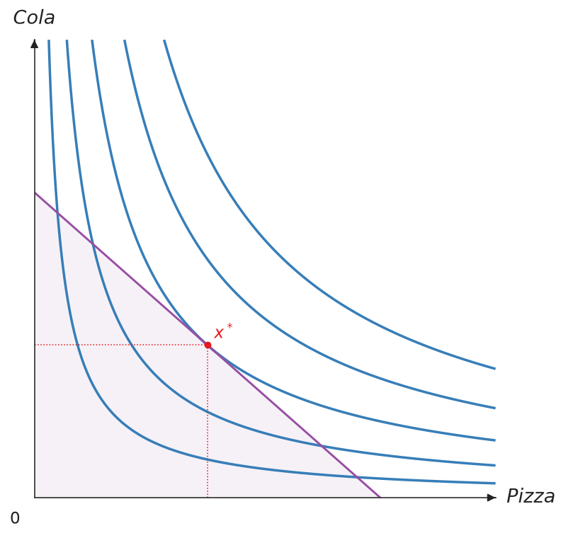Before — every level has the same visual weight.
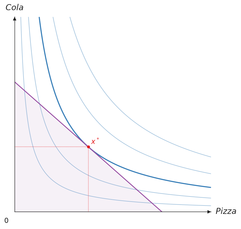After — the equilibrium level is focal.
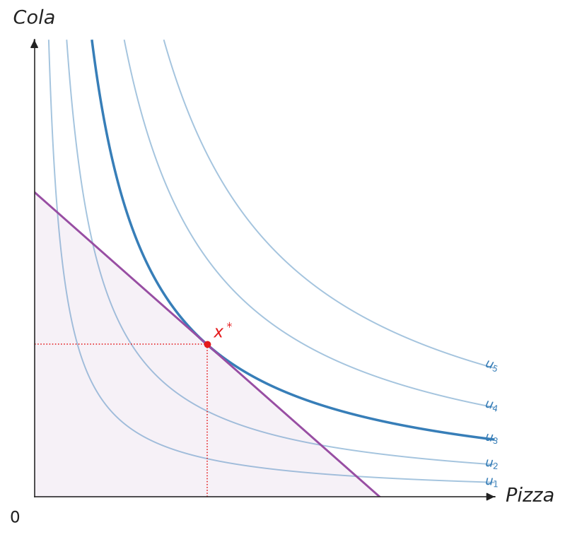Ordinal labels — curves are labelled \(u_1,u_2,\ldots\).

Budget line

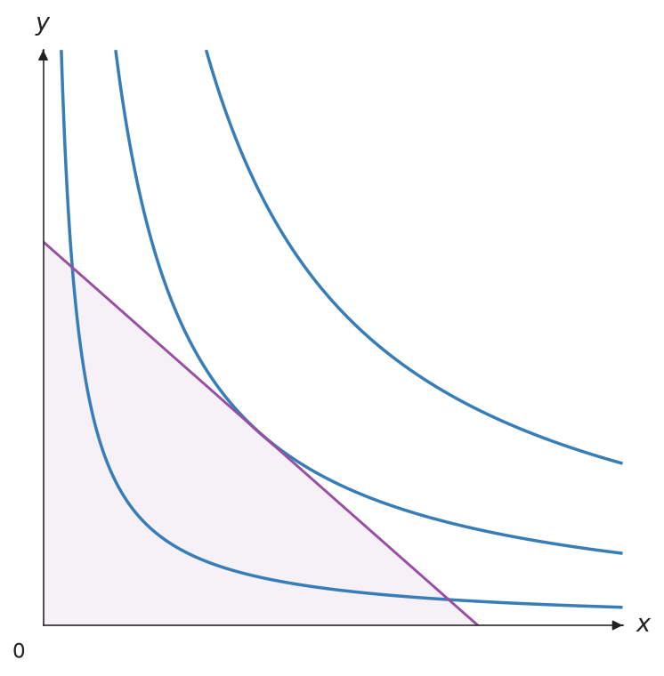
Draws the budget line \(p_x x + p_y y = I\). Set fill=True to shade the feasible set below it.

cvs.add_budget(
    px, py, income,
    stroke=None,       # default: theme.budget_stroke
    label=None,        # legend label (LaTeX)
    fill=False,        # True, or a Fill; default: theme.budget_fill
)

Budget line with the shaded feasible set

Equilibrium

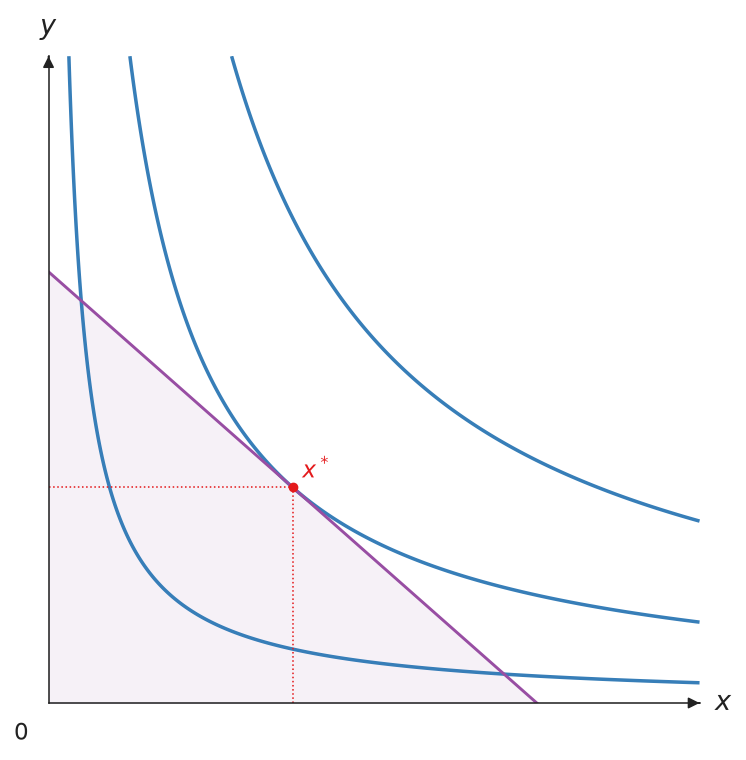
Marks the optimal bundle and drops dashed lines to both axes. Pass the result of solve() as eq; show_ray=True also draws the expansion path through the origin.

cvs.add_equilibrium(
    eq,                # result of solve()
    label="x^*",       # str or Label
    marker=None,       # default: theme.eq_marker
    drop_dashes=True,  # dashed lines to axes
    show_ray=False,    # expansion path
    drop_stroke=None,
    ray_stroke=None,
)

Equilibrium point with dashed drop lines

Ray

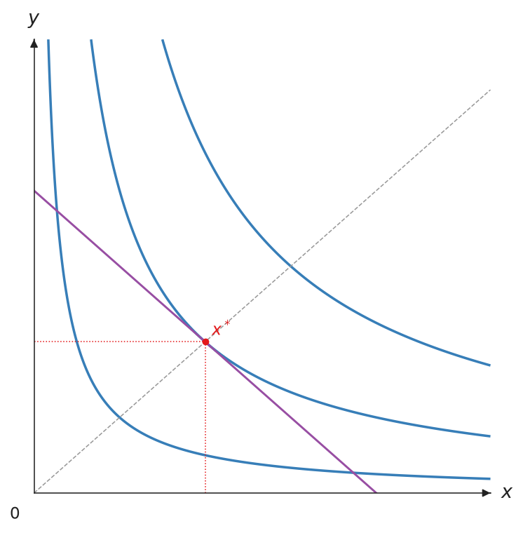
Draws a dashed ray from the origin with slope slope (dy/dx), often used for an expansion path or a fixed consumption ratio.

cvs.add_ray(
    slope,             # dy/dx
    stroke=None,       # default: theme.ray_stroke
)

Expansion-path ray through the optimum

Point

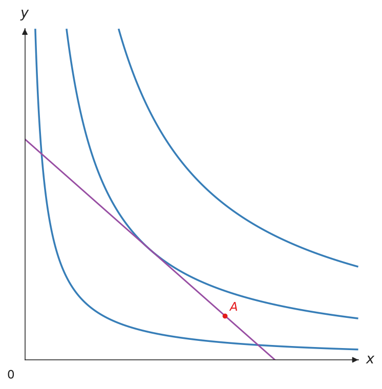
Marks any point, such as a bundle to compare with the optimum. label is rendered in LaTeX math mode; pass a Label to move or restyle it.

cvs.add_point(
    x, y,
    label=None,        # str or Label
    marker=None,       # default: theme.point_marker
)

Labelled point A on the budget line

Show and save

show() opens an interactive window. save() infers the format from the file extension: .png, .pdf, .svg, or .tex for TikZ. It also releases matplotlib resources, so call it last.

cvs.show()               # interactive window
cvs.save("figure.png")   # .png / .pdf / .svg / .tex

Complete diagram ready to save

Styles

Each kind of element has its own style object. Fields left as None keep the theme default, so set only what you want to change.

Object	Styles	Theme defaults
`Stroke`	Line width, line style, colour, arrowhead	`theme.budget_stroke`, `theme.ic_stroke`, …
`Marker`	Point colour, size, shape	`theme.eq_marker`, `theme.point_marker`, …
`Label`	Text, position, offset, colour, size, visibility	`theme.point_label`, `theme.axis_label`, …
`Legend`	Legend position, size, frame, columns	`theme.legend`
`Fill`	Shading colour and opacity	`theme.budget_fill`
`Axis`	One axis's label, label position, and stroke	none

Every object also takes an opacity from 0 (transparent) to 1 (opaque).

from econ_viz import Canvas, Fill, Label, Marker, Stroke

(
    Canvas(x_max=20, y_max=15)
    .add_utility(model, levels=lvls, ic_label=Label(text="U={:.1f}", position="top"))
    .add_budget(2.0, 3.0, 30.0, stroke=Stroke(color="black"),
                fill=Fill(color="lightgrey", opacity=0.4))
    .add_equilibrium(eq, marker=Marker(color="#C0392B", shape="s"),
                     label=Label(position="bottom-left", offset=8))
    .add_point(12.0, 2.0, label=Label(text="A", position="left"))
    .save("styles.png")
)

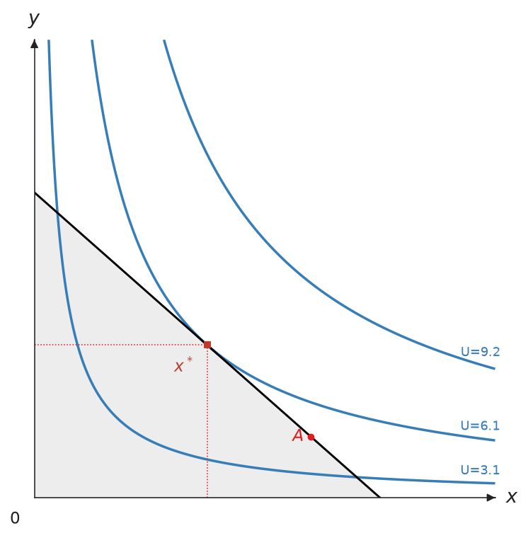
Custom stroke, fill, markers, and labels

Stroke is the preferred way to style lines. The separate color, linewidth, and linestyle arguments still work as shorthand and draw the same thing. A label takes its point's Marker colour unless it sets its own; label positions are top, bottom, left, right, and the four corners such as top-right, and Label(visible=False) hides a label.

Text and legend

Every piece of text takes a Label: axis labels through Axis(label=...), the origin through origin_label, and the title through title. Legends go where they cover the least of the diagram, moving outside the plot area when every corner is taken; a Legend chooses an inside corner ("upper left", …) or a side outside ("top", "bottom", "left", "right").

from econ_viz import Axis, Canvas, Label, Legend

cvs = Canvas(
    title=Label(text="Cobb-Douglas", fontsize=13),
    x_axis=Axis(label=Label(text="x_1", fontsize=16)),
    origin_label=Label(visible=False),
)
cvs.show_legend(legend=Legend(position="bottom", fontsize=10))

The line and arrow styles below apply to the axes with the x_* and y_* parameters, and to any other line through Stroke.

Line styles

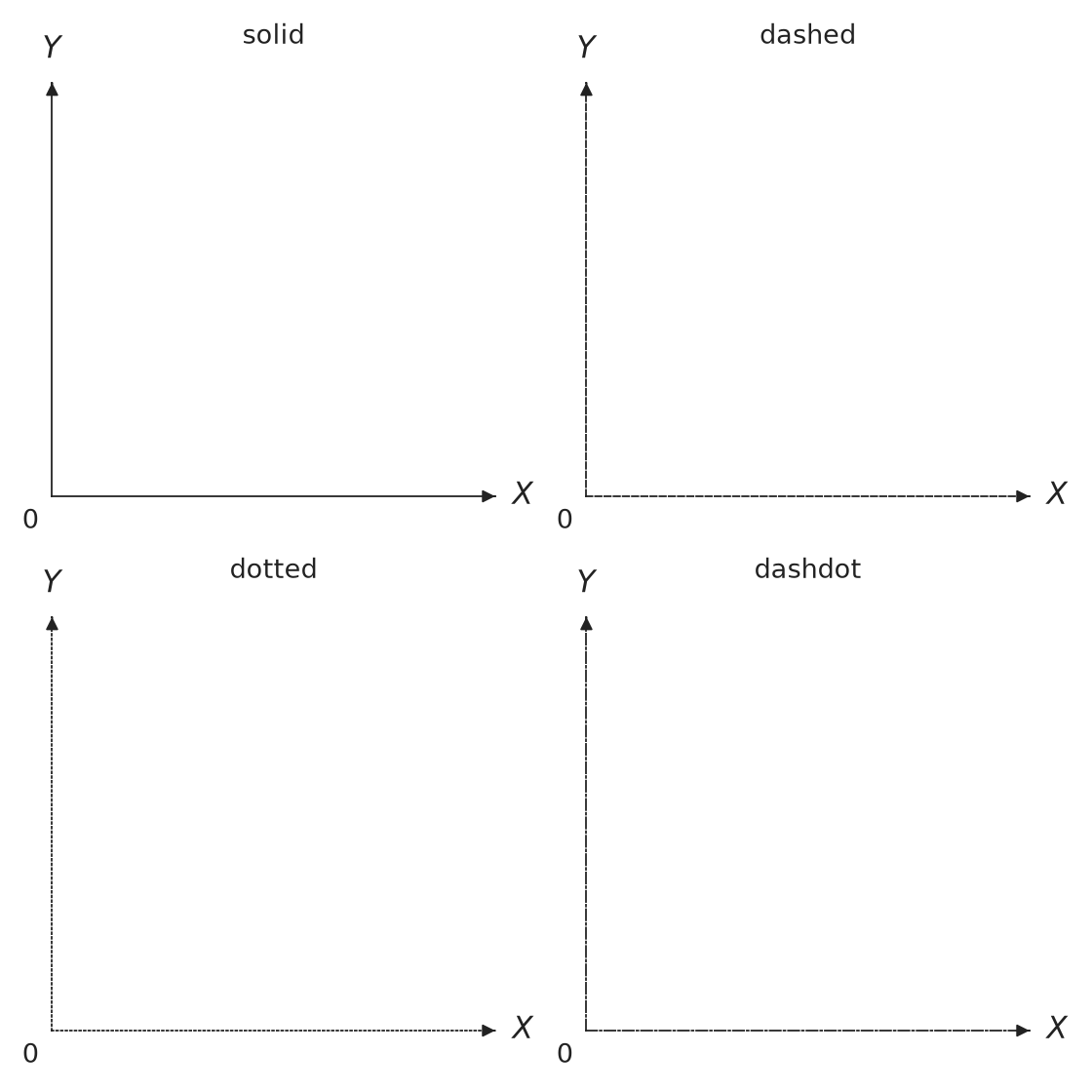
Use LineStyle.SOLID, DASHED, DOTTED, or DASHDOT for axis lines. The equivalent strings—solid, dashed, dotted, and dashdot—are also accepted. Use Stroke(style=...) to apply the same setting to any other line.

import matplotlib.pyplot as plt

from econ_viz import Canvas, LineStyle

styles = [
    LineStyle.SOLID,
    LineStyle.DASHED,
    LineStyle.DOTTED,
    LineStyle.DASHDOT,
]

fig, axes = plt.subplots(2, 2, figsize=(7, 7))
for ax, style in zip(axes.flat, styles):
    Canvas(
        title=style.value,
        x_line_style=style,
        y_line_style=style,
        fig=fig,
        ax=ax,
    )

fig.tight_layout()
fig.savefig("line_styles.png", dpi=160, transparent=True)

Available line styles

Arrow styles

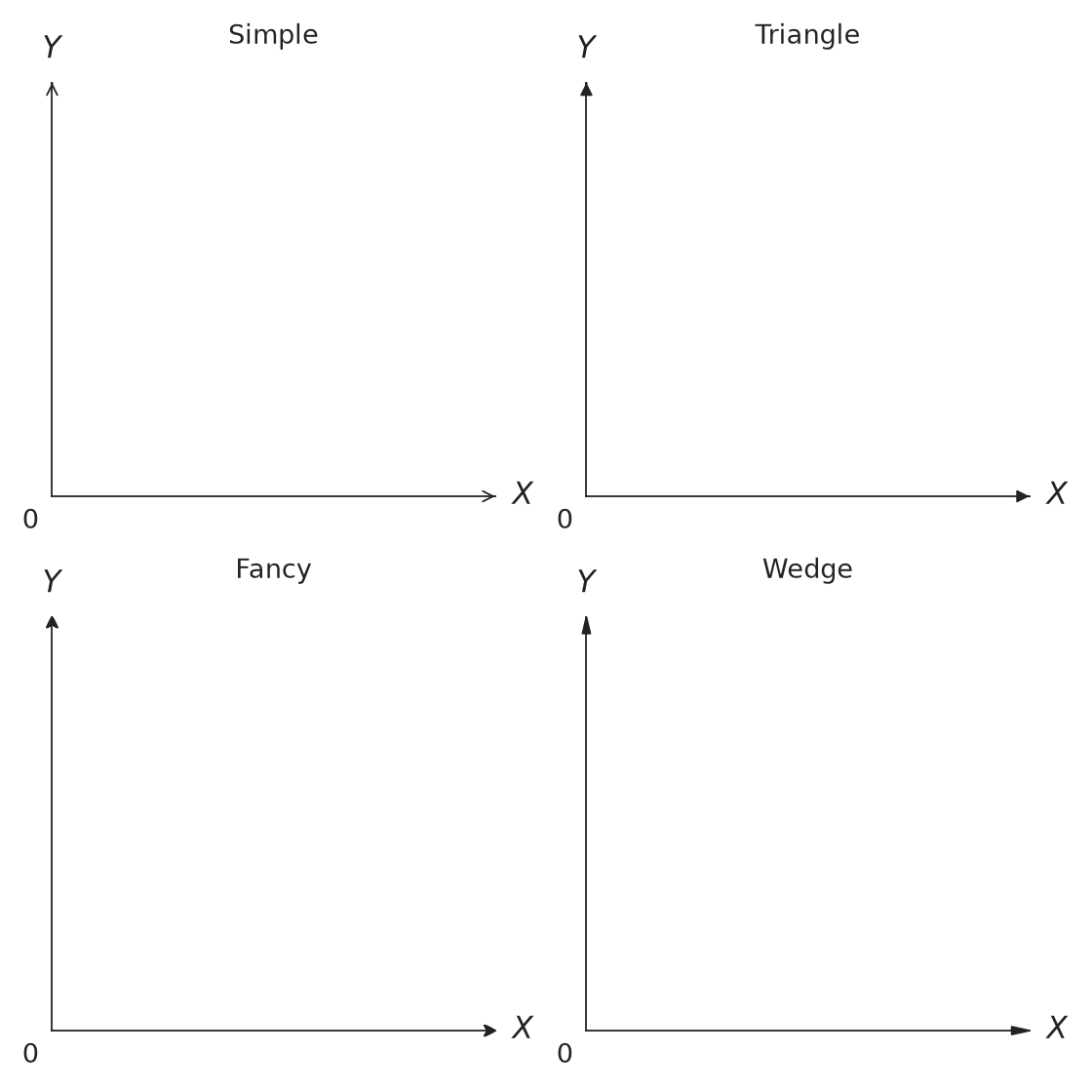
Use ArrowStyle.SIMPLE, TRIANGLE, FANCY, or WEDGE for axis arrowheads. Use Stroke(arrow=...) to add the same arrowhead to another visible line.

import matplotlib.pyplot as plt

from econ_viz import ArrowStyle, Canvas

styles = [
    ArrowStyle.SIMPLE,
    ArrowStyle.TRIANGLE,
    ArrowStyle.FANCY,
    ArrowStyle.WEDGE,
]

fig, axes = plt.subplots(2, 2, figsize=(7, 7))
for ax, style in zip(axes.flat, styles):
    Canvas(
        title=style.name.title(),
        x_arrow_style=style,
        y_arrow_style=style,
        fig=fig,
        ax=ax,
    )

fig.tight_layout()
fig.savefig("arrow_styles.png", dpi=160, transparent=True)

Available arrow styles

Stroke is also available for paths, decomposition diagrams, DemandDiagram, Figure, and EdgeworthBox. Fields left as None inherit from the active theme.

Method chaining

Canvas(x_max=20, y_max=15) \
    .add_utility(model, levels=lvls) \
    .add_budget(2.0, 3.0, 30.0, fill=True) \
    .add_equilibrium(eq, show_ray=True) \
    .save("figure.png")