Core Models

The core models cover smooth preferences, kinked and linear preferences, and preferences with income or reference-point effects. Choose a group, then switch between its tabs to compare models.

Smooth preferences

These models produce smooth indifference curves and normally have an interior optimum when prices and income are positive.

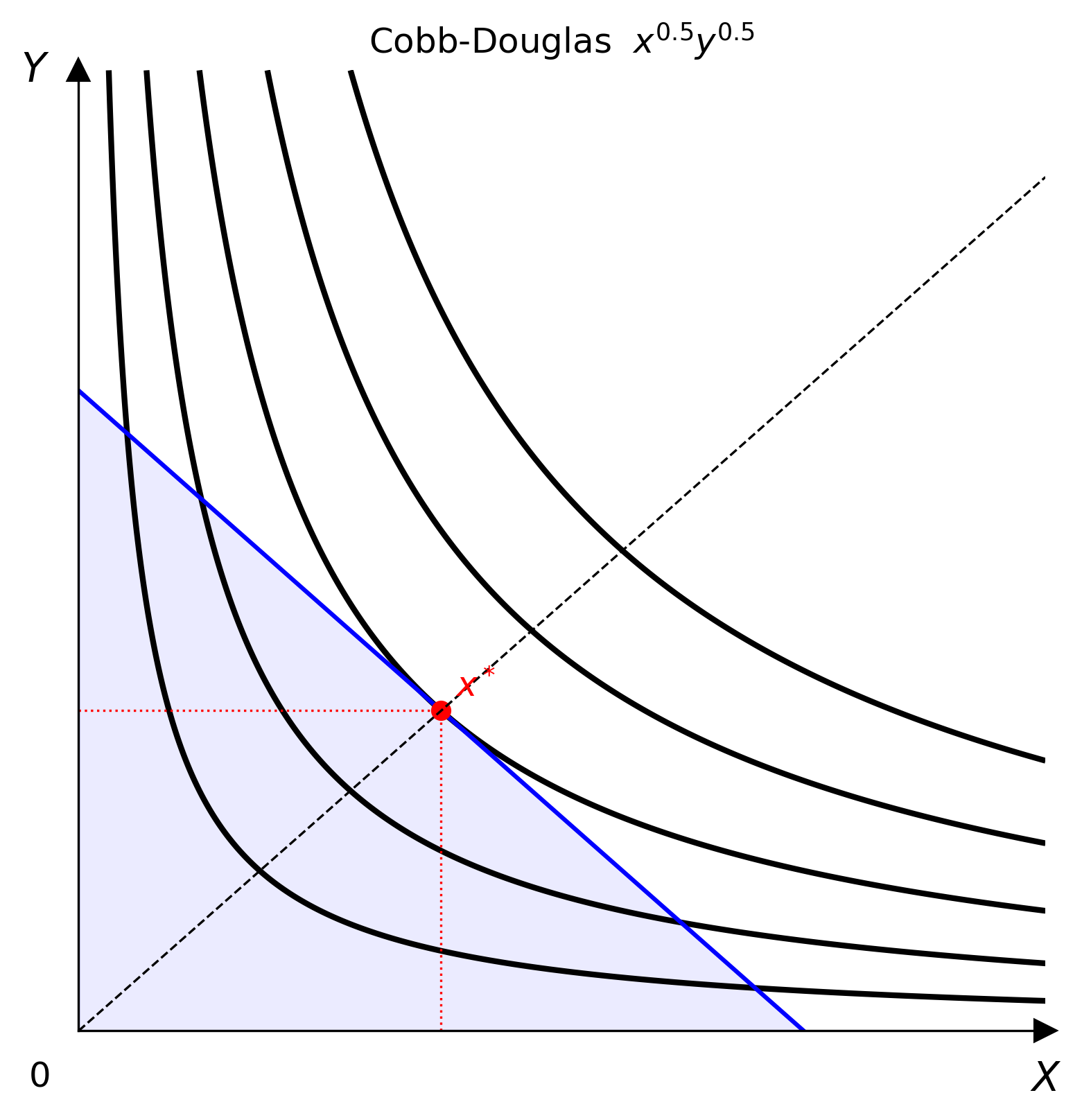
Cobb-DouglasCESTranslog

Cobb-Douglas is the standard model for smooth, strictly convex preferences.

\[ U(x,y)=x^\alpha y^\beta \]

The exponents control the relative weight placed on each good. Its indifference curves approach both axes without touching them.

Parameters

Parameter	Default	Meaning
`alpha`	`0.5`	Weight on good \(x\)
`beta`	`0.5`	Weight on good \(y\)

Example

from econ_viz import Canvas, levels, solve
from econ_viz.models import CobbDouglas

model = CobbDouglas(alpha=0.5, beta=0.5)
eq = solve(model, px=2.0, py=3.0, income=30.0)

(
    Canvas(x_max=20, y_max=15, title="Cobb-Douglas")
    .add_utility(model, levels=levels.around(eq.utility, n=5))
    .add_budget(2.0, 3.0, 30.0, fill=True)
    .add_equilibrium(eq, show_ray=True)
    .save("cobb_douglas.png")
)

Cobb-Douglas indifference map

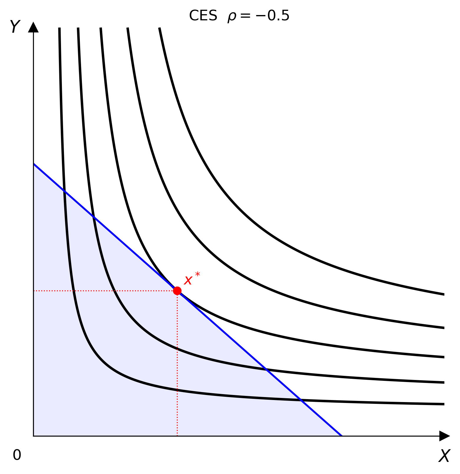
CES lets the ease of substitution vary while keeping preferences smooth.

\[ U(x,y)=\left(\alpha x^\rho+\beta y^\rho\right)^{1/\rho} \]

The substitution elasticity is \(\sigma=1/(1-\rho)\). As \(\rho\) changes, CES approaches Cobb-Douglas, Leontief, or perfect substitutes.

Parameters

Parameter	Default	Meaning
`alpha`	`0.5`	Weight on good \(x\)
`beta`	`0.5`	Weight on good \(y\)
`rho`	`0.5`	Substitution parameter, with \(\rho\ne1\)

Example

from econ_viz import Canvas, levels, solve
from econ_viz.models import CES

model = CES(alpha=0.5, beta=0.5, rho=-0.5)
eq = solve(model, px=2.0, py=3.0, income=30.0)

(
    Canvas(x_max=20, y_max=15, title="CES")
    .add_utility(model, levels=levels.around(eq.utility, n=5))
    .add_budget(2.0, 3.0, 30.0)
    .add_equilibrium(eq)
    .save("ces.png")
)

CES indifference map

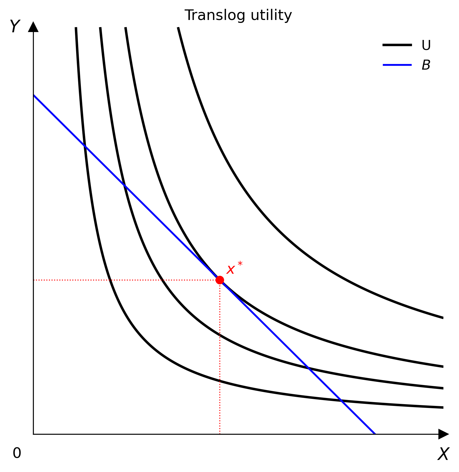
Translog is a flexible log-quadratic model for smooth preferences.

\[ \begin{aligned} \ln U(x,y)={}&\alpha_0+\alpha_x\ln x+\alpha_y\ln y\\ &+\tfrac12\beta_{xx}(\ln x)^2 +\tfrac12\beta_{yy}(\ln y)^2 +\beta_{xy}\ln x\ln y \end{aligned} \]

The quadratic and interaction terms allow curvature to vary across the consumption space. Setting all \(\beta\) coefficients to zero gives a Cobb-Douglas-style log-linear form.

Parameters

Parameter	Default	Meaning
`alpha_0`	`0.0`	Log-utility intercept
`alpha_x`	`0.5`	First-order weight on \(\ln x\)
`alpha_y`	`0.5`	First-order weight on \(\ln y\)
`beta_xx`	`0.0`	Curvature in \(x\)
`beta_yy`	`0.0`	Curvature in \(y\)
`beta_xy`	`0.0`	Interaction between \(x\) and \(y\)

Example

from econ_viz import Canvas, levels, solve
from econ_viz.models import Translog

model = Translog(alpha_x=0.6, alpha_y=0.4, beta_xy=0.12)
eq = solve(model, px=2.0, py=3.0, income=30.0)

(
    Canvas(x_max=18, y_max=12, title="Translog")
    .add_utility(model, levels=levels.around(eq.utility, n=4))
    .add_budget(2.0, 3.0, 30.0)
    .add_equilibrium(eq)
    .save("translog.png")
)

Translog indifference map

Kinks and corners

These models show how non-smooth or linear preferences change the location of the optimum.

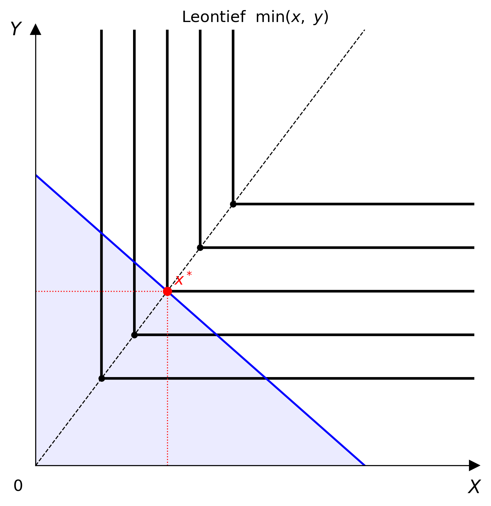
LeontiefPerfect SubstitutesMaximum Utility

Leontief preferences describe goods consumed in fixed proportions.

\[ U(x,y)=\min(ax,by) \]

Indifference curves are L-shaped. The optimum lies at the kink where the two weighted quantities are equal.

Parameters

Parameter	Default	Meaning
`a`	`1.0`	Weight on good \(x\)
`b`	`1.0`	Weight on good \(y\)

Example

from econ_viz import Canvas, levels, solve
from econ_viz.models import Leontief

model = Leontief(a=1.0, b=1.0)
eq = solve(model, px=2.0, py=3.0, income=30.0)

(
    Canvas(x_max=20, y_max=15, title="Leontief")
    .add_utility(
        model,
        levels=levels.around(eq.utility, n=5),
        show_rays=True,
        show_kinks=True,
    )
    .add_budget(2.0, 3.0, 30.0)
    .add_equilibrium(eq)
    .save("leontief.png")
)

Leontief indifference map

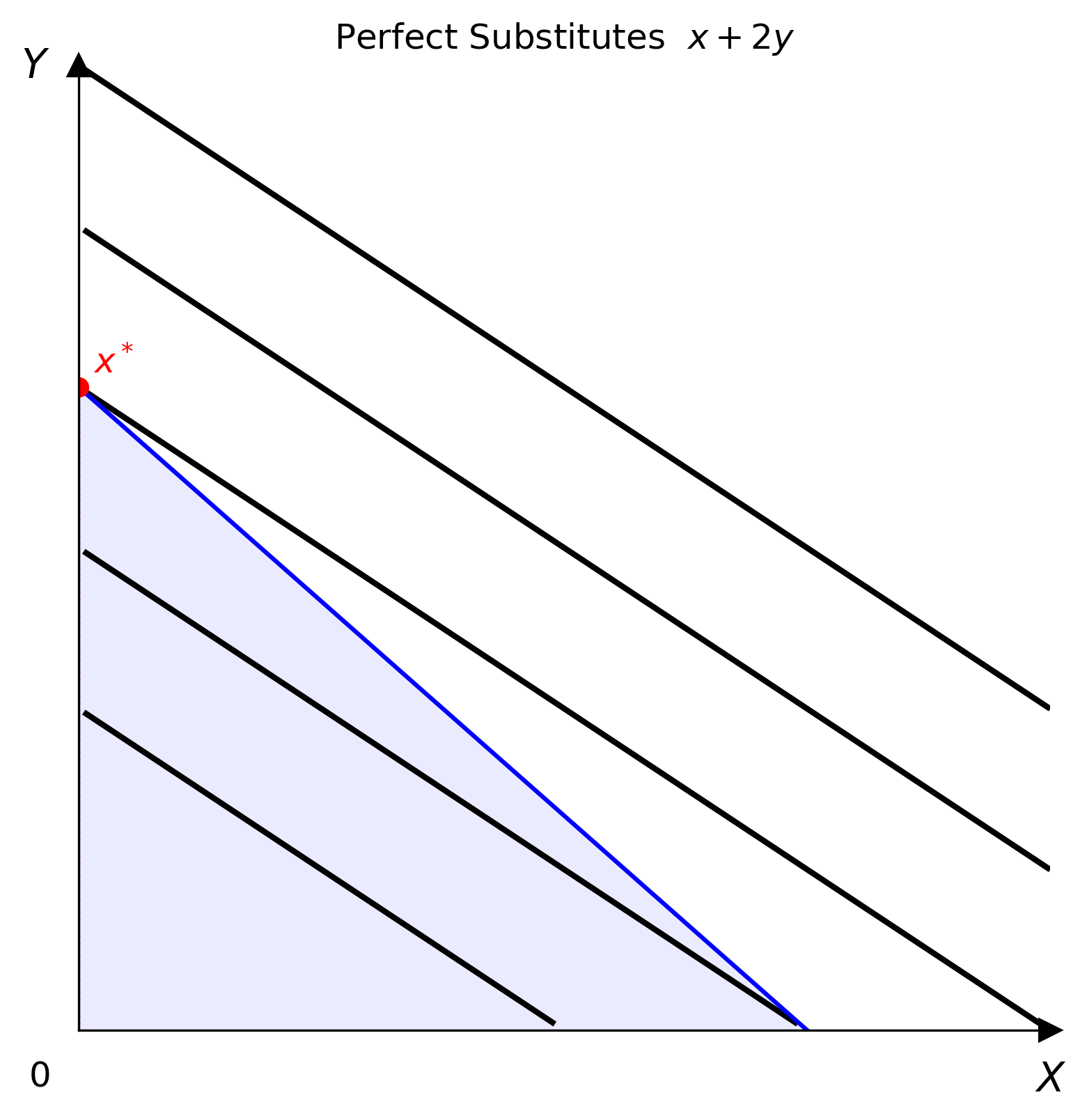
Perfect substitutes provide constant utility trade-offs between goods.

\[ U(x,y)=ax+by \]

Indifference curves are straight lines. The consumer normally chooses the good with the greater marginal utility per dollar, producing a corner solution.

Parameters

Parameter	Default	Meaning
`a`	`1.0`	Marginal utility of good \(x\)
`b`	`1.0`	Marginal utility of good \(y\)

Example

from econ_viz import Canvas, levels, solve
from econ_viz.models import PerfectSubstitutes

model = PerfectSubstitutes(a=1.0, b=2.0)
eq = solve(model, px=2.0, py=3.0, income=30.0)

(
    Canvas(x_max=20, y_max=15, title="Perfect Substitutes")
    .add_utility(model, levels=levels.around(eq.utility, n=5))
    .add_budget(2.0, 3.0, 30.0)
    .add_equilibrium(eq)
    .save("perfect_substitutes.png")
)

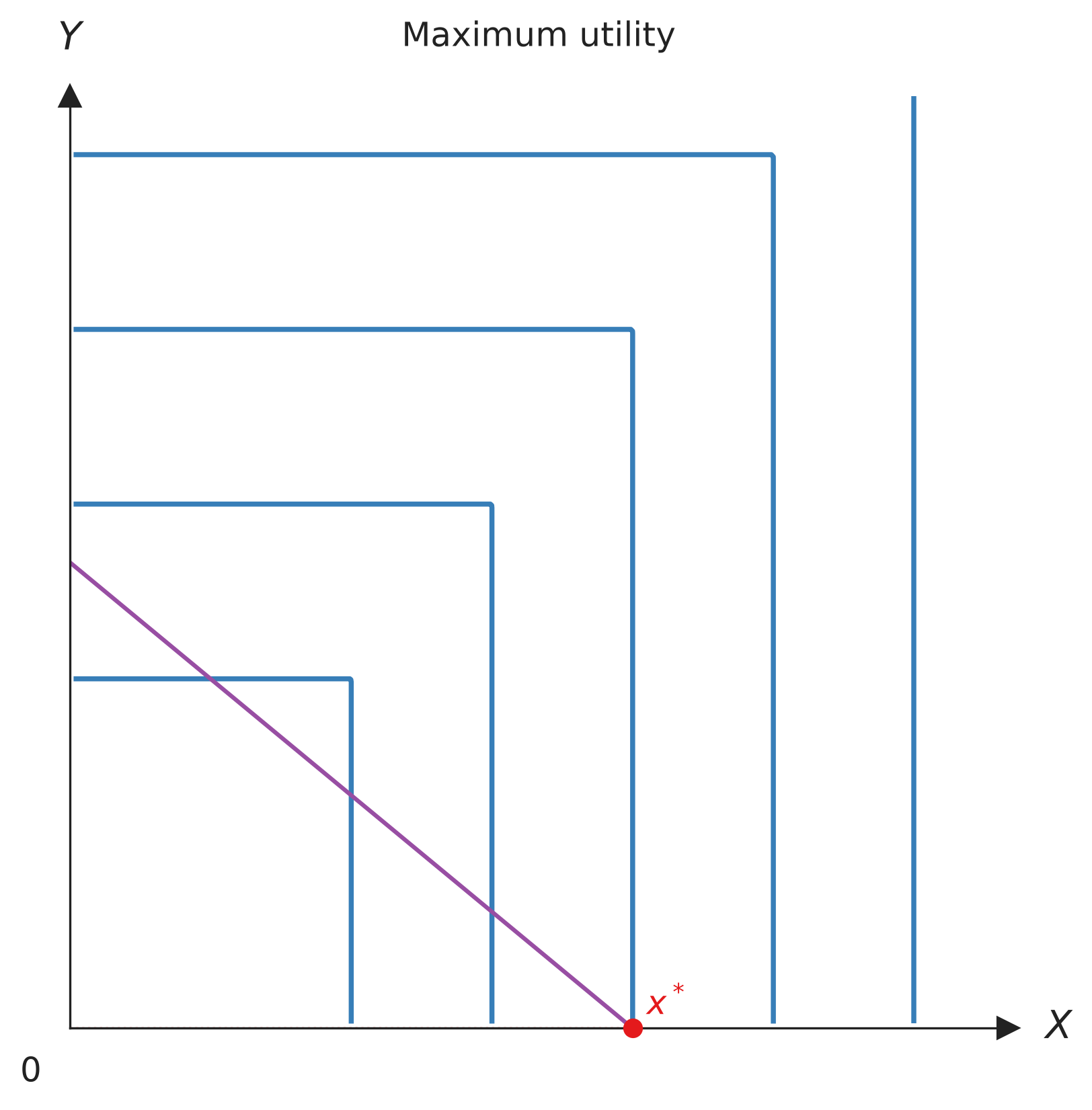
Perfect Substitutes indifference map

Maximum utility keeps only the larger weighted quantity in each bundle.

\[ U(x,y)=\max(ax,by) \]

Each indifference curve has two arms that extend toward the axes. The resulting preferences are non-convex, so the optimum on a linear budget normally lies at the intercept with the greater weighted utility.

Parameters

Parameter	Default	Meaning
`a`	`1.0`	Weight on good \(x\)
`b`	`1.0`	Weight on good \(y\)

Example

import numpy as np
from econ_viz import Canvas, levels, solve
from econ_viz.models import CustomUtility

a, b = 1.0, 1.0
model = CustomUtility(
    func=lambda x, y: np.maximum(a * x, b * y),
    name="maximum",
)
eq = solve(model, px=2.0, py=3.0, income=30.0)

(
    Canvas(x_max=25, y_max=20, title="Maximum utility")
    .add_utility(model, levels=levels.around(eq.utility, n=5))
    .add_budget(2.0, 3.0, 30.0)
    .add_equilibrium(eq)
    .save("maximum.png")
)

Maximum utility indifference map

Income and reference points

These models add special income effects, subsistence requirements, or a preferred consumption point.

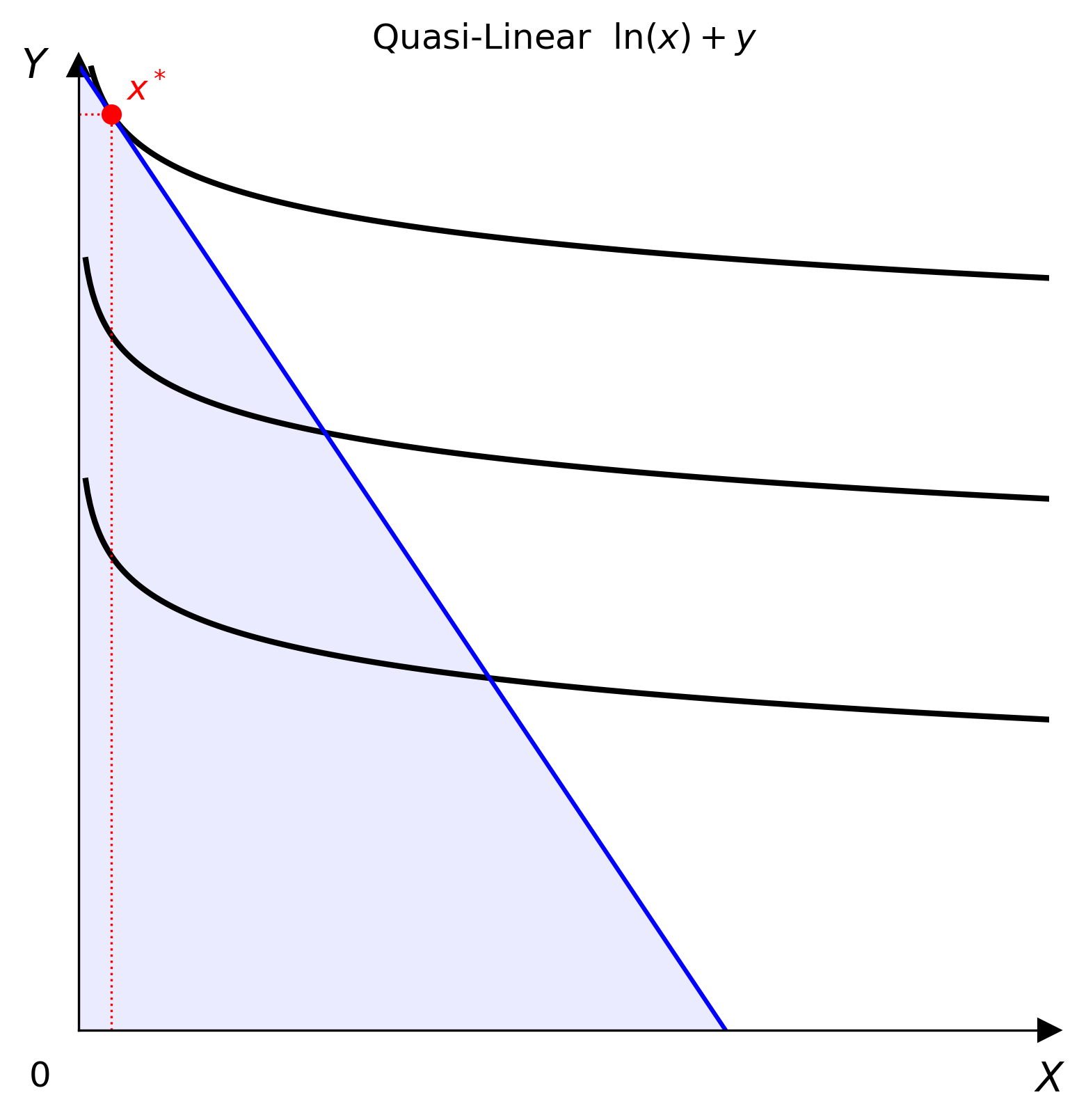
Quasi-LinearStone-GearySatiation

Quasi-linear preferences place one good linearly in utility.

\[ U(x,y)=f(x)+y \]

The non-linear good has no income effect once the solution is interior. linear_in can reverse the roles of \(x\) and \(y\).

Parameters

Parameter	Default	Meaning
`v_func`	`numpy.log`	Increasing, concave function \(f\)
`linear_in`	`"y"`	Good that enters linearly

Example

import numpy as np
from econ_viz import Canvas, levels, solve
from econ_viz.models import QuasiLinear

model = QuasiLinear(v_func=np.log, linear_in="y")
eq = solve(model, px=2.0, py=1.0, income=20.0)

(
    Canvas(x_max=15, y_max=15, title="Quasi-Linear")
    .add_utility(model, levels=levels.around(eq.utility, n=5))
    .add_budget(2.0, 1.0, 20.0)
    .add_equilibrium(eq)
    .save("quasi_linear.png")
)

Quasi-Linear indifference map

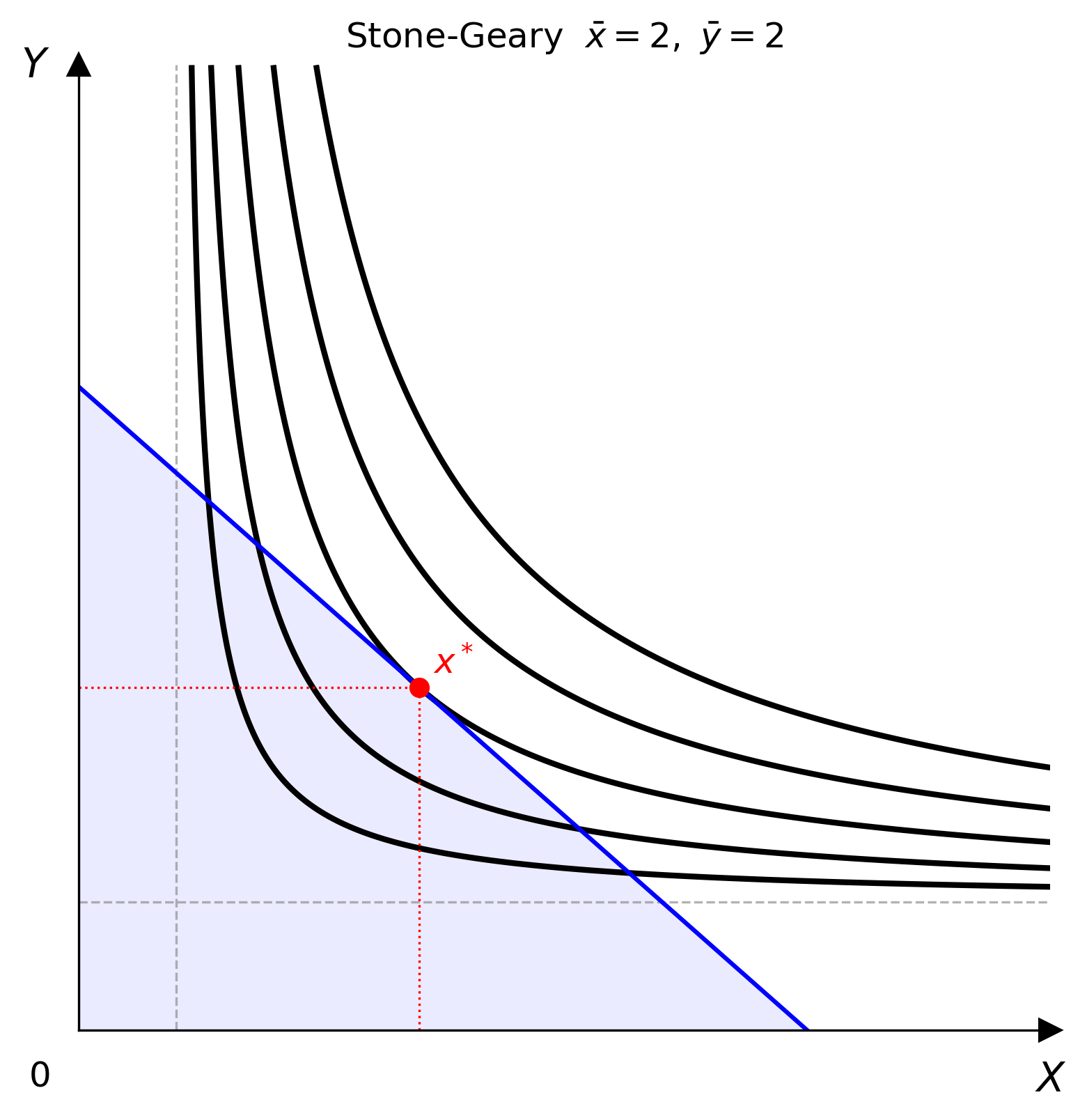
Stone-Geary extends Cobb-Douglas with minimum consumption requirements.

\[ U(x,y)=(x-\bar{x})^\alpha(y-\bar{y})^\beta \]

The consumer first covers subsistence quantities \(\bar{x}\) and \(\bar{y}\), then allocates the remaining income like a Cobb-Douglas consumer.

Parameters

Parameter	Default	Meaning
`alpha`	`0.5`	Weight on supernumerary \(x\)
`beta`	`0.5`	Weight on supernumerary \(y\)
`bar_x`	`1.0`	Subsistence quantity \(\bar{x}\)
`bar_y`	`1.0`	Subsistence quantity \(\bar{y}\)

Example

from econ_viz import Canvas, levels, solve
from econ_viz.models import StoneGeary

model = StoneGeary(alpha=0.5, beta=0.5, bar_x=2.0, bar_y=2.0)
eq = solve(model, px=2.0, py=3.0, income=30.0)

(
    Canvas(x_max=20, y_max=15, title="Stone-Geary")
    .add_utility(model, levels=levels.around(eq.utility, n=5))
    .add_budget(2.0, 3.0, 30.0, fill=True)
    .add_equilibrium(eq)
    .save("stone_geary.png")
)

Stone-Geary indifference map

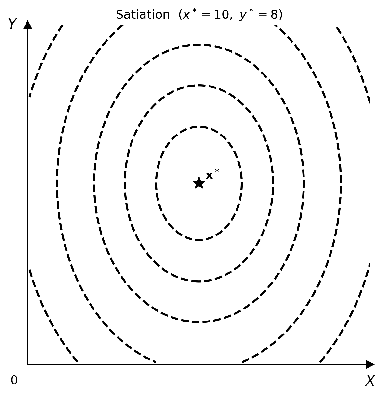
Satiation preferences have a bliss point that maximises utility.

\[ U(x,y)=-a(x-x^*)^2-b(y-y^*)^2 \]

Utility falls in every direction away from \((x^*,y^*)\), so indifference curves form closed ellipses and monotonicity does not hold.

Parameters

Parameter	Default	Meaning
`bliss_x`	`5.0`	Bliss-point coordinate \(x^*\)
`bliss_y`	`5.0`	Bliss-point coordinate \(y^*\)
`a`	`1.0`	Curvature along the \(x\)-axis
`b`	`1.0`	Curvature along the \(y\)-axis

Example

import numpy as np
from econ_viz import Canvas, levels
from econ_viz.models import Satiation

model = Satiation(bliss_x=6.0, bliss_y=4.0)
x = np.linspace(0.1, 12.0, 300)
y = np.linspace(0.1, 10.0, 300)
X, Y = np.meshgrid(x, y)

(
    Canvas(x_max=12, y_max=10, title="Satiation")
    .add_utility(model, levels=levels.percentile(model(X, Y), n=5))
    .save("satiation.png")
)

Satiation indifference map

For custom functions and multi-good Cobb-Douglas models, see Advanced Models.

Core Models

Smooth preferences

Kinks and corners

Income and reference points

Comments