Quick Start

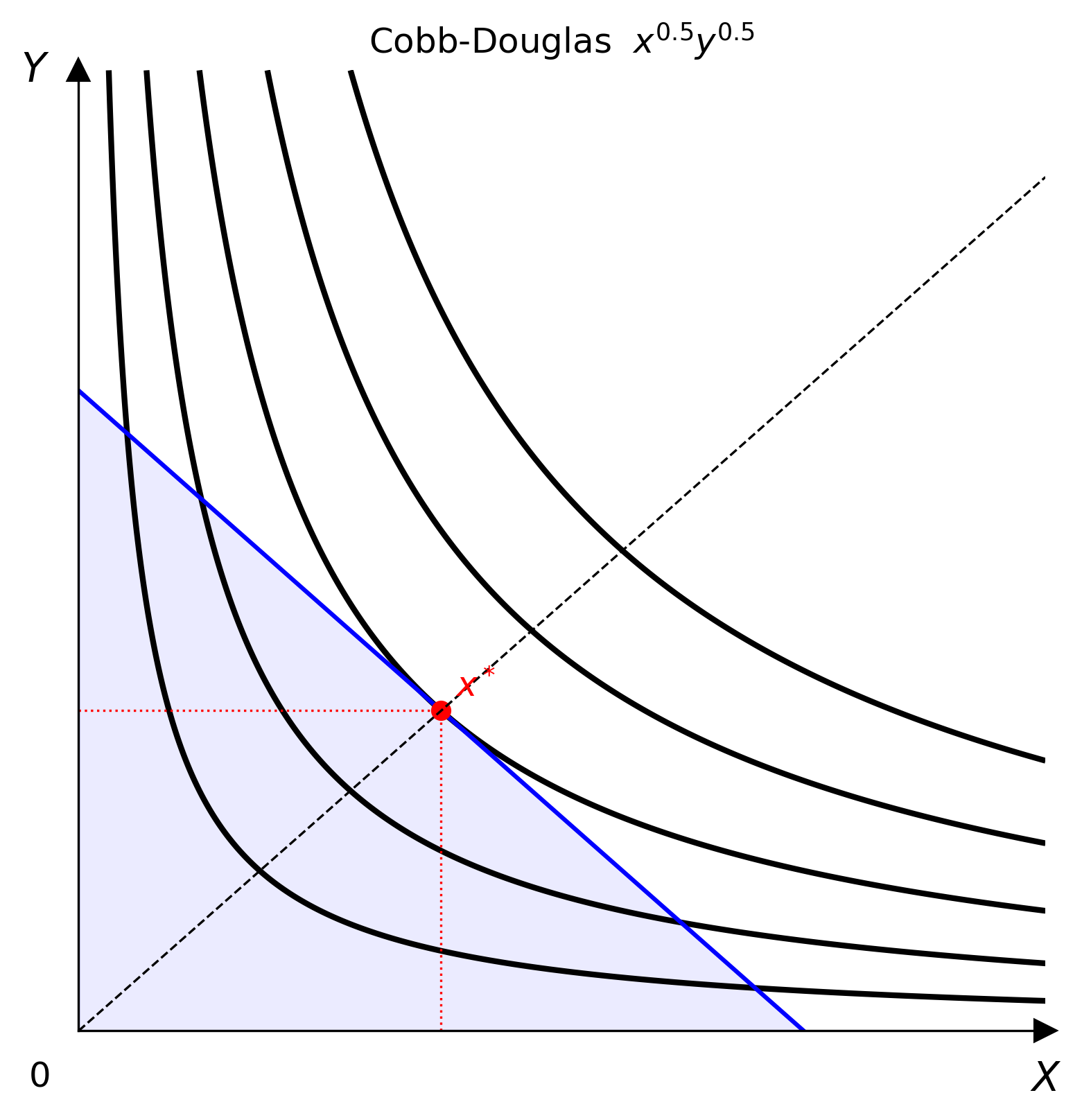
Minimal example

from econ_viz import Canvas, levels, solve
from econ_viz.models import CobbDouglas

model = CobbDouglas(alpha=0.5, beta=0.5)
eq    = solve(model, px=2.0, py=3.0, income=30.0)
lvls  = levels.around(eq.utility, n=5)

cvs = Canvas(x_max=20, y_max=15, x_label="x", y_label="y",
             title=r"Cobb-Douglas $x^{0.5} y^{0.5}$")
cvs.add_utility(model, levels=lvls)
cvs.add_budget(2.0, 3.0, 30.0, fill=True)
cvs.add_equilibrium(eq, show_ray=True)
cvs.save("cobb_douglas.png")

Step by step

Choose a model

Pick a utility function from econ_viz.models. See the Model catalogue for the full list.

from econ_viz.models import CobbDouglas
model = CobbDouglas(alpha=0.5, beta=0.5)

Solve for the equilibrium

solve() returns an Equilibrium named tuple with fields x, y, utility, and bundle_type.

from econ_viz import solve
eq = solve(model, px=2.0, py=3.0, income=30.0)
print(eq.x, eq.y, eq.utility)   # e.g. 7.5  5.0  5.303

Choose indifference-curve levels

from econ_viz import levels
lvls = levels.around(eq.utility, n=5)   # 5 curves centred on the optimum

Build the canvas

from econ_viz import Canvas
cvs = Canvas(x_max=20, y_max=15)

Add layers

Canvas methods return self, so calls can be chained:

cvs.add_utility(model, levels=lvls)
cvs.add_budget(2.0, 3.0, 30.0, fill=True)
cvs.add_equilibrium(eq, show_ray=True)

Export

Raster / vectorInteractive

cvs.save("figure.png")    # PNG
cvs.save("figure.pdf")    # PDF
cvs.save("figure.svg")    # SVG

cvs.show()   # opens a live matplotlib window

Using the LaTeX parser

from econ_viz import parse_latex, Canvas, levels, solve

model = parse_latex(r"x^{0.4} y^{0.6}")
eq    = solve(model, px=2.0, py=3.0, income=30.0)
lvls  = levels.around(eq.utility, n=5)

Canvas(x_max=20, y_max=15) \
    .add_utility(model, levels=lvls) \
    .add_budget(2.0, 3.0, 30.0) \
    .add_equilibrium(eq) \
    .save("figure.png")

Multi-panel figures

Figure lets you compose several Canvas panels into one layout.

from econ_viz import Figure, Layout, levels, solve
from econ_viz.models import CobbDouglas

fig = Figure(
    Layout.SIDE_BY_SIDE,
    x_max=20,
    y_max=15,
    x_label="x",
    y_label="y",
    title="Before / After Price Change",
    shared_y=True,
)

cases = [
    (CobbDouglas(alpha=0.5, beta=0.5), 2.0, 3.0, 30.0, r"Before: $p_x=2$"),
    (CobbDouglas(alpha=0.3, beta=0.7), 4.0, 3.0, 30.0, r"After: $p_x=4$"),
]

for idx, (model, px, py, income, title) in enumerate(cases):
    eq = solve(model, px=px, py=py, income=income)
    panel = fig[idx]
    panel.ax.set_title(title)
    panel.add_utility(model, levels=levels.around(eq.utility, n=5))
    panel.add_budget(px, py, income, fill=True)
    panel.add_equilibrium(eq, show_ray=True)

fig.save("comparison.png")

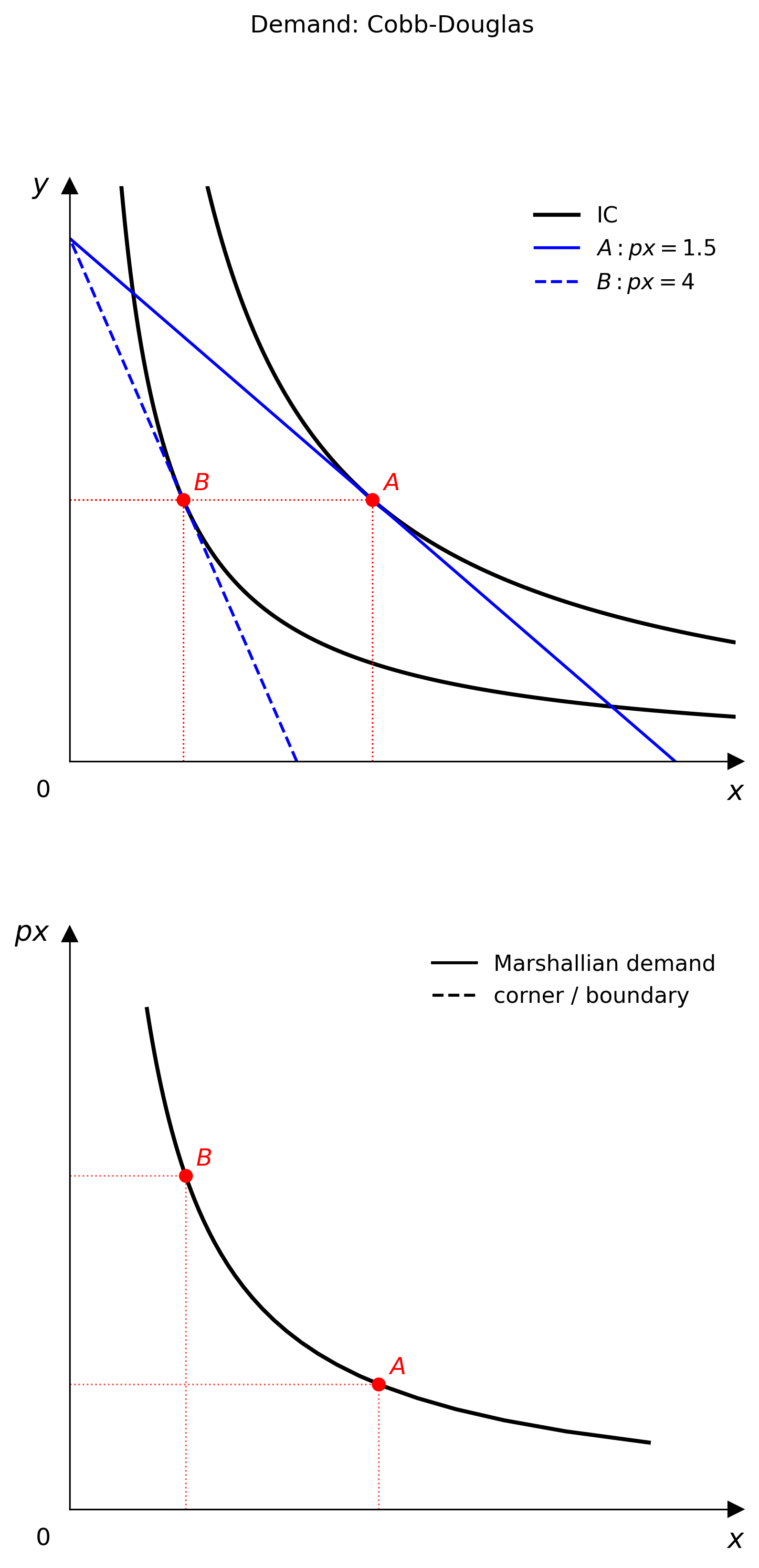
Demand diagrams

Use PricePath plus DemandDiagram to link the goods-space optimum to Marshallian demand.

from econ_viz import DemandDiagram, LinearBudget, PricePath
from econ_viz.models import CobbDouglas

model = CobbDouglas(alpha=0.5, beta=0.5)
budget = LinearBudget(px=2.0, py=2.0, income=40.0)
path = PricePath(model, budget=budget, price="px", price_range=(0.8, 6.0), n=40)

fig = DemandDiagram(path, title="Demand: Cobb-Douglas")
fig.add_marshallian_panel(price_markers=[1.5, 4.0])
fig.save("demand.png")

Comments